Prediction of an Additive
Manufacturing Defect Based on Deep Learning

Wang, Lidong

doi:10.70322/ism.2025.10014

Intelligent and Sustainable Manufacturing

Submit to ISM

Article Open Access

Prediction of an Additive Manufacturing Defect Based on Deep Learning

Lidong Wang ^*

Author Information

Institute for Systems Engineering Research, Mississippi State University, Vicksburg, MS 39180, USA

Authors to whom correspondence should be addressed.

Views:200

Downloads:24

Intelligent and Sustainable Manufacturing 2025, 2 (1), 10014; https://doi.org/10.70322/ism.2025.10014

Received: 04 March 2025 Accepted: 10 April 2025 Published: 18 April 2025

ABSTRACT: Selective laser melting (SLM) is one of the additive manufacturing (AM) methods and the most studied laser-based AM process for metals and alloys. The optimization of the laser process parameters of SLM and the prediction of defects such as cracks, keyholes, and lack of fusion (LOF) are significant for improving the product quality of SLM. Deep learning (DL) has the potential to analyze complex processes and predict anomalies; however, much data is generally needed for training a DL model. Experimental studies on AM, such as SLM, often use the design of experiments (DOE) to reduce the number of experiments and save costs and time. Therefore, much experimental data is not prepared to create the DL model. This paper deals with creating a DL model on a small experimental data set with unbalanced data and predicting the defect LOF of SLM using the created DL model. Data analytics is performed based on four DL methods, including the Elman neural network, the Jordan neural network, the deep neural network (DNN) with weights initialized by the deep belief network (DBN), and the regular DNN based on the algorithms ‘rprop+’ and ‘sag’. It is shown that the regular DNN based on the ‘sag’ algorithm, after the z-score standardization of the small data set, helps create an accurate DL model and achieve good analytics and prediction results. The three other DL methods in this paper do not work well on the small data set (with unbalanced data) in the defect prediction.

Keywords: Additive manufacturing; Selective laser melting; Deep learning; Deep neural network; Defect; Prediction

1. Introduction

Additive manufacturing (AM) is also called 3D printing. It has been used in aeronautical and astronautical industries, the automobile industry, the healthcare industry, etc. SLM is one of the AM methods. Sometimes, micro-defects form during the manufacturing process of SLM. A method for real-time monitoring of the forming of micro-defects during the SLM process was developed using proprietary battery-powered equipment that enables continuous recording and wireless transmission of acoustic emission waveforms. This method monitored micro-cracks and pores generated during the SLM process in real-time [1]. One of the challenges in the SLM of metals is controlling the formation of keyhole pores due to a local excessive energy input during the SLM process. Monitoring and controlling the formation of defects during the SLM process can reduce or avoid degraded mechanical properties (resulting from the defects) and permit circumvention of time-consuming and costly post-process stages. A method of performing in-situ healing of deep keyhole pores was developed using a positively defocused laser beam with finely tuned remelting process parameters [2]. Precise control of the SLM process of polymers is important to guarantee the structural integrity of automotive and aerospace parts. Machine learning (ML) was used to predict local porosity or solidity based on thermal and temporal features extracted from the melt’s temperature-time profile. The in-situ process signature was measured employing infrared thermography, and the porosity analysis was performed by X-ray micro-computed tomography [3]. Although physics-based and data-driven methods are effective, they have limitations in interpretability, generalizability, and accuracy for the complicated process optimization and prediction solutions of a metal AM process. Physics-informed ML was developed recently, in which physics knowledge (such as thermomechanical theories and constraints) was infused into ML models to achieve interpretability, reliability, and improved predictive efficiency and accuracy of created models [4]. Defect detection based on computed tomography (CT) images plays a significant role in developing metallic AM. Although some deep learning (DL) methods have been used in CT image-based defect detection, there are still challenges in accurately detecting small defects, especially if there is undesirable noise. A depth-connected region-based convolutional neural network (CNN) was developed to reduce the influence of noise and accurately detect small-sized defects [5]. A simultaneous multi-step model predictive control (MPC) framework was developed for real-time decision-making based on a multivariate DNN. Directed energy deposition (DED) (one of the AM methods) was used as a case study, and it was demonstrated that the proposed MPC is effective in tracking the melt pool temperature to ensure part quality while reducing porosity defects by regulating the laser power [6]. DL [7] is a subset of ML. There are more hidden layers in a DL network than in a traditional artificial neural network (ANN). DL can automatically learn and discover relevant features from data or examples (cases/instances); therefore, it can detect patterns and trends and make predictions. DL can handle large data, and generally, much data is needed for training a DL model. A DL model can improve its performance if more data is available and used for model training. Overfitting and data availability are two major challenges in DL. Overfitting leads to poor performance on new data. Generally, it is necessary to collect/gather quality data (such as balanced data, not biased data, etc.) for DL model training; however, large amounts of data in engineering are often not available. For example, experimental studies on SLM often use the design of experiments (DOE) to reduce the number of experiments and save costs and time. Therefore, much of the experimental data of SLM is for specific tasks; it is not prepared for DL and the DL model creation. The work in this paper is part of the author’s effort to explore a DL model on a small experimental data set with unbalanced data. The purpose of the research in this paper is to create a DL model on a small data set with unbalanced data and perform the prediction of a defect (LOF) of SLM using the created DL model. The remainder of this paper will be organized as follows: the second section introduces SLM; the third section presents data, data pre-processing methods, and evaluation metrics for DL; the fourth section introduces DL methods used in this paper, including Elman networks and Jordan networks, deep neural networks (DNN) with weights initialized by the deep belief network, and regular DNN based on the algorithms ‘rprop+’ and ‘sag’; the fifth section presents results and discussion; and the sixth section is the conclusion and future work.

2. Selective Laser Melting

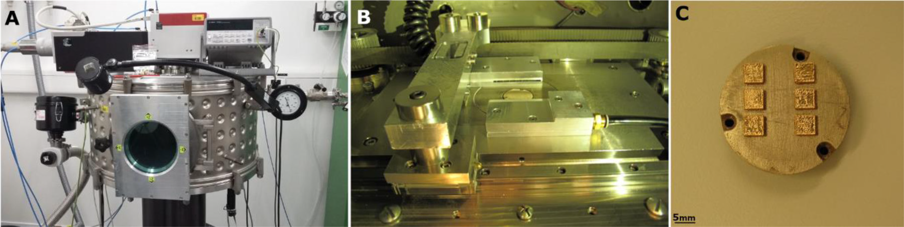
Laser powder bed fusion (LPBD), or SLM, is the most studied laser-based AM process for metals and alloys. Figure 1 illustrates an in-house SLM machine, a printing plate, powder deposition, a gas flow system, and an example of SLM-produced bronze samples. A significant issue in SLM is the time-consuming identification of a process window leading to quasi-fully dense parts (>99.8%), commonly based on trials and errors [8].

Figure 1. (A) An in-house SLM machine, (B) a printing plate, powder deposition, and gas flow system, and (C) an example of SLM-produced bronze samples [8].

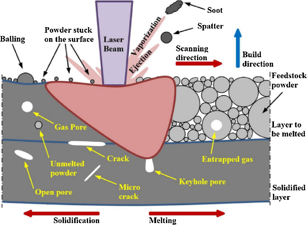
An experimental study on metallurgical issues related to the SLM of stainless steel 316 L and Invar 36 was conducted. A full factorial design of experiments (DOE) was designed, and different laser process parameters were tested. When energy is below a critical value, a lack of fusion (LOF)/unmelted powder was observed due to insufficient melt tracks and discontinuous beads. SLM products can exhibit stress risers and some dislocations, as illustrated in Figure 2. There can be highly localized changes in both the heating rate during the powder melting of SLM and the cooling rate during the part solidification process of SLM. The thermal changes can lead to changes in the composition, variations in the thermal expansion, and void formation. The optimization of the laser process parameters of SLM should be fulfilled in the early stage of the SLM process to avoid stress risers, reduce defects, and improve product quality [9].

Figure 2. SLM melt pool formation with some possible defects [9].

3. Data, Data Pre-Processing Methods, and Evaluation Metrics for Deep Learning

The Nickel-based powder superalloy Ni-13Cr-4Al-5Ti has exceptional performance at high temperatures. The SLM of the superalloy and related defects were studied successfully, and significant results were achieved. The major defects include cracks, keyholes, and lack of fusion (LOF). The laser process parameters include the laser power (W), the scanning speed (mm/s), the hatch space (mm), and the scanning rotation (°) [10]. This paper focuses on the defect of LOF. The original experimental data of the SLM of the superalloy (Ni-13Cr-4Al-5Ti) includes 52 rows and 5 columns (only LOF is used for deep learning in this paper). In the column of the scanning rotation, there are five ‘0’ values, five ‘45’ values, 32 ‘67’ values, five ‘90’ values, and five ‘180’ values. There is unbalanced data in this column. Therefore, the data set is small and has unbalanced data. In the column of LOF, ‘yes’ is set to 1, and ‘no’ is set to 0 for deep learning. There are 30 ‘1’ values and 20 ‘0’ values. The experimental data was not prepared for DL although it was not necessary for DL training and testing. Table 1 only shows partial experimental data of the SLM of the superalloy.

Table 1. Partial experimental data of SLM [10].

No.	Power (W)	Speed (mm/s)	Hatch Space (mm)	Rotation (°)	Lack of Fusion (LOF)
1	200	1000	0.06	45	Yes (1)
2	200	2200	0.15	180	Yes (1)
3	240	1400	0.12	180	Yes (1)
4	240	1800	0.15	0	Yes (1)
5	270	1700	0.05	67	Yes (1)
6	270	1900	0.07	67	Yes (1)
7	280	2200	0.06	90	Yes (1)
8	280	600	0.09	180	Yes (1)
9	280	1400	0.15	45	Yes (1)
10	290	1800	0.05	67	Yes (1)
11	290	1900	0.06	67	Yes (1)
12	320	1400	0.03	90	Yes (1)
13	320	2200	0.09	0	Yes (1)
14	360	1000	0.03	180	Yes (1)
15	360	600	0.15	90	Yes (1)
16	200	600	0.03	0	No (0)
17	240	1000	0.09	90	No (0)
18	270	1800	0.05	67	No (0)
19	270	1700	0.07	67	No (0)
20	280	1900	0.05	67	No (0)
21	280	1700	0.07	67	No (0)
22	290	1900	0.05	67	No (0)
23	290	1700	0.06	67	No (0)
24	320	600	0.12	45	No (0)
25	320	1000	0.15	67	No (0)

Two common methods to normalize (or “scale”) variables are:

: Min-max normalization: (X − min(X))/(max(X) − min(X))
: Z-score standardization: (X − μ)/σ

where X is the data values, μ is the mean, and σ is the standard deviation. A random sampling with a 70-30 split or 80-20 split on a large and quality database is often used for DL model training and testing. In this paper, a random sampling with a 60-40 split on the small data set is performed because there are only 20 ‘0’s in total in the data set. It means that the training data are chosen through a random sampling of 60% of instances in the dataset, and the remaining instances (40%) after the sampling are utilized for testing. Choosing a 70-30 split or an 80-20 split on the small data set will lead to a small number of test data and a poor performance evaluation (e.g., an unideal accuracy value). Choosing a 60-40 split on the small data set increases the amount of test data. There are two classes (‘Yes’ and ‘No’, or ‘1’ and ‘0’) in the above data set. One class can be treated as ‘positive’ (its value = 1) while the other can be treated as ‘negative’ (its value = 0). True positive (TP), false positive (FP), true negative (TN), and false negative (FN) are described as follows [11]: TP: the number of positive cases correctly classified as positive. FP: the number of negative cases incorrectly classified as positive. TN: the number of negative cases correctly classified as negative. FN: the number of positive cases incorrectly classified as negative. The accuracy (ACC), false positive rate (FPR), and false negative rate (FNR) are employed as measures for the classification and the performance of DL methods in this paper. They are calculated utilizing the following formulas [12,13,14]:

```latexA C C = \left( T P + T N \right) / \left( T P + F P + T N + F N \right)```

(1)

```latexF P R = \left( F P \right) / \left( F P + T N \right)```

(2)

```latexF N R = \left( F N \right) / \left( F N + T P \right)```

(3)

The value of (TP + FP + TN + FN) is the total number of cases or instances in the test data of the dataset. Traditional ML methods (e.g., traditional ANN) have been used to predict the LoF defect. The results (e.g., an accuracy of 42.86%) obtained are not good (far from acceptable), or no results are obtained due to the convergence problem, which is the expected situation due to the dataset characteristics (small and unbalanced, see Table 1). Generally, this kind of data is also not appropriate for DL and the creation of the DL model. However, DL is generally more powerful (e.g., handling complex data) than traditional ML methods. The objective of the research in this paper is to explore a DL model on a small experimental dataset with unbalanced data, predict the LoF defect using the created DL model, and improve the modeling and prediction performance (according to the accuracy, FPR, and FNR).

4. Deep Learning Methods

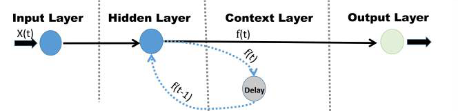
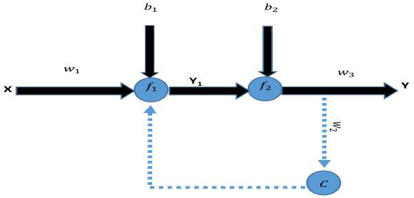
4.1. Elman Networks and Jordan Networks Both Elman networks and Jordan networks are recurrent neural networks (RNNs). A simple form of an RNN is shown in Figure 3. An Elman neural network has one or more context layers. In the Elman neural network, the number of neurons in the context layer is equal to the number of neurons in the hidden layer. Furthermore, the context layer neurons are fully connected to all the neurons in the hidden layer. Jordan networks are like Elman neural networks. The only difference is that the context neurons in Jordan networks are fed from the output layer instead of the hidden layer (in Elman networks), which is shown in Figure 4 [15]. An Elman network can be considered a model constantly unfolding as a sequence of predictors. A Jordan network uses a context layer to process sequential data [15]. The data set (see Table 1) used in this paper is experimental data that can be regarded as a sequential data set over time.

Figure 3. A simple recurrent neural network [15].

Figure 4. A simple Jordan network [15].

The Elman neural network and the Jordan neural network can be described as follows [16,17]:

```latexh_{t} = \sigma_{h} \left( W_{h} x_{t} + U_{h} h_{t - 1} + b_{h} \right) \, \mathrm{for\, the \,Elman\, network}```

(4)

```latexh_{t} = \sigma_{h} \left( W_{h} x_{t} + U_{h} y_{t - 1} + b_{h} \right) \, \mathrm{for \,the \,Jordan \,network}```

(5)

```latexy_{t} = \sigma_{y} \left( W_{y} h_{t} + b_{y} \right)```

(6)

where $$x_t$$ is the input vector that is the input vector $$V=(V_1,V_2,…,V_p)$$ in this paper, $$h_t$$ is the hidden layer vector, $$y_t$$ is the output vector; W, U, and b are the parameter matrices and vectors; and $$σ_h$$ and $$σ_y$$ are activation functions. 4.2. Deep Neural Networks with Weights Initialized by the Deep Belief Network A deep neural network (DNN) with weights initialized by a deep belief network (DBN) means the DNN with the initial values of its weights that are set utilizing the learned features from a pre-trained DBN. This method is named DNN-DBN in this paper. The potential advantages of utilizing DBN for the initialized weights lie in the capability of processing complex data, good generalization, and enhanced training speed. A DBN can be viewed as a composition of restricted Boltzmann machines (RBMs). The procedures of DNN with weights initialized by DBN include (1) training a DBN, (2) extracting weights (extracting the learned weights from hidden layers as soon as the training of DBN is finished), (3) initializing the DNN, and (4) performing “fine-tune” with supervised learning. An RBM-based DBN was utilized as a pre-trainer to initialize the weights of a DNN. The pre-trained DNN was fine-tuned [18]. The proper parameter initialization in a DNN based on the DBN was studied and examined. It was shown that DBN can be utilized to decide the initial DNN parameters, weights, and biases. This method outperforms the only DNN used method in most cases [19]. The training method for RBMs is called contrastive divergence (CD) [20]. Pre-training and fine-tuning are performed during the training of a DBN. The following is some specific information on the method and algorithm [21,22]. The “energy” of a network can be written as $$E \left(v , h\right) .$$ $$p \left(v\right)$$ is the probability of a visible vector, and it is written as follows:

```latexp \left(v\right) = \frac{1}{Z} \underset{h}{\sum} e^{- E \left( v , h \right)}```

(7)

where $$Z = \sum \exp ⁡ \left( - E \left(v , h\right)\right)$$ is the partition function. For training an RBM, weights can be updated as follows:

```latexw_{i j} \left(t + 1\right) = w_{i j} \left(t\right) + \eta \cdot \frac{\partial l o g \left( p \left( v \right) \right)}{\partial w_{i j}}```

(8)

4.3. Regular Deep Neural Networks In deep neural network (DNN) learning [23,24], each training tuple can be processed in two steps [23]: propagating the inputs forward and backpropagating the error. For an input vector $$V = \left( V_{1} , V_{2} , \ldots , V_{p} \right)$$, each hidden layer transforms its input vector from the layer to the next layer by employing an affine transform and nonlinear mapping as follows:

```latexz^{\left( 1 \right)} = V```

(9)

```latexy_{j}^{\left( l \right)} = \sum\nolimits_{j = 1}^{N^{\left( l \right)}} w_{i j}^{\left( l \right)} z_{i}^{\left( l - 1 \right)} + \theta_{j}^{\left( l \right)} \,\,\,\,\,\,\, \left(l = 2, 3,\ldots, L\right) ```

(10)

```latexz_{j}^{\left( l \right)} = f \left( y_{j}^{\left( l \right)} \right)```

(11)

where L is the total number of layers; $$N^{\left( l \right)}$$, $$\theta_{j}^{\left( l \right)}$$, and $$w_{i j}^{\left( l \right)}$$ are the number of units in the lth layer, the bias of the unit j in the lth layer, and the weight of the connection from unit i in the previous layer to unit j of the lth layer, respectively; and f is a nonlinear activation function. In this paper, Elman networks and Jordan networks, DNN with weights initialized by the deep belief network, and regular DNN based on the algorithms ‘rprop+’ and ‘sag’ are used to create DL models and perform the prediction of a defect (LOF) of SLM because all of the DL methods achieved good accuracy, FNR, and FPR when large and quality databases such as ‘spambase’ (it is publicly available online and can be downloaded from the following website: https://archive.ics.uci.edu/mL/datasets/Spambase (accessed on 16 April 2025)) were used in my previous research. The two algorithms ‘rprop+’ and ‘sag’ worked well on ‘spambase’. ‘rprop+’ refers to the resilient back-propagation with weight backtracking; ‘sag’ induces the usage of the modified globally convergent algorithms.

5. Results and Discussion

5.1. Results of Elman Networks and Jordan Networks Both Elman networks and Jordan networks are recurrent neural networks (RNNs), and they can be used to analyze sequential data sets. Table 2 and Table 3 show the results of the Elman and Jordan networks with min-max normalization and z-score standardization, respectively. They show that the Elman networks and Jordan networks do not work well in the creation of DL models on the small data set (with unbalanced data) and the prediction of the defect LOF of the SLM. The accuracy (ACC) values are low, and the FPR values, as well as the FNR values, are high. The reason lies in the small data set and the unbalanced data in the dataset. The structures of context layers show the number of nodes in the context layers. For example, c(6) means six nodes are in the context layer.

Table 2. Data analytics based on Elman networks and Jordan networks with data normalization (min-max normalization).

Algorithms or Methods	Structures (Context Layers)	FPR (%)	FNR (%)	ACC (%)
Elman	c(4)	62.50	30.77	57.14
Elman	c(6)	62.50	46.15	47.62
Jordan	c(4)	75.00	38.46	47.62
Jordan	c(6)	62.50	23.08	61.90

Table 3. Data analytics based on Elman networks and Jordan networks with z-score standardization.

Algorithms or Methods	Structures (Context Layers)	FPR (%)	FNR (%)	ACC (%)
Elman	c(4)	87.50	53.85	33.33
Elman	c(6)	75.00	53.85	38.10
Jordan	c(4)	75.00	38.46	47.62
Jordan	c(6)	50.00	38.46	57.14

5.2. Results of DNNs with Weights Initialized by the DBN Table 4 and Table 5 show the results of the DNNs with weights initialized by the DBN when min-max normalization and z-score standardization are utilized, respectively. It is shown that this method does not work well in the creation of DL models on the small dataset (with unbalanced data) and the prediction of the defect LOF. Besides the input layer and the output layer, two or three hidden layers are used, and the performance (according to the accuracy, FPR, and FNR) of the created DL models is not good. The reason lies in the small data set and unbalanced data. The structures of hidden layers show the number of nodes in the hidden layers. For example, c(10, 8, 4) means there are three hidden layers, and the numbers of nodes in the three hidden layers are 10, 8, and 4, respectively. In Table 4, n/a indicates that no normal result can be obtained if structure c(10, 8, 4) is adopted and min-max normalization is employed.

Table 4. Data analytics based on DNN-DBN with data normalization (min-max normalization).

Algorithms

or Methods

Structures

(Hidden Layers)

FPR

(%)

FNR

(%)

ACC

(%)

DNN-DBN

c(10, 4)

87.50

23.08

52.38

c(12, 6)

87.50

15.38

57.14

c(10, 8, 4)

n/a

Table 5. Data analytics based on DNN-DBN with z-score standardization.

Algorithms or Methods	Structures (Hidden Layers)	FPR (%)	FNR (%)	ACC (%)
DNN-DBN	c(10, 4)	12.50	53.85	61.90
	c(12, 6)	12.50	53.85	61.90
	c(6, 3, 2)	25.00	30.77	71.43
	c(10, 8, 4)	25.00	46.15	61.90

5.3. Results of Regular DNNs The results of regular DNNs created on the small data set (with unbalanced data) of the SLM are shown in Table 6 (without data normalization), Table 7 (min-max normalization), and Table 8 (with z-score standardization). Table 6 indicates that the regular DNN based on the algorithm ‘rprop+’ achieves better results than the above three DL methods (Elman, Jordan, and DNN-DBN) when the hidden layer structure c(16, 12, 4) is adopted, even if no data normalization is employed. When z-score standardization is employed, the regular DNN based on the algorithm ‘rprop+’ achieves 85.71% accuracy when the hidden layer structure c(6, 4, 2) is adopted, and the regular DNN based on the algorithm ‘sag’ achieves 90.48% accuracy when the hidden layer structure c(6, 3, 2) is adopted. The structure c(6, 3, 2) means there are five layers in the deep neural network, including the input layer, three hidden layers, and the output layer. The number of nodes in the first hidden layer, the second hidden layer, and the third hidden layer is 6, 3, and 2, respectively. The relevant FPR and FNR values of the two accuracy values are much lower than those of the three DL methods (Elman, Jordan, and DNN-DBN).

Table 6. Data analytics based on regular DNNs without data normalization.

Algorithms	Structures (Hidden Layers)	FPR (%)	FNR (%)	ACC (%)
rprop+	c(16, 10, 4)	75.00	23.08	57.14
rprop+	c(16, 12, 4)	75.00	0.00	71.43
sag	c(16, 10, 4)	0.00	92.31	42.86
sag	c(16, 12, 4)	75.00	15.38	61.90

Table 7. Data analytics based on regular DNNs with data normalization (min-max normalization).

Algorithms	Structures (Hidden Layers)	FPR (%)	FNR (%)	ACC (%)
rprop+	c(16, 10, 4)	12.50	38.46	71.43
rprop+	c(16, 12, 4)	12.50	38.46	71.43
sag	c(16, 10, 4)	12.50	69.23	52.38
sag	c(16, 12, 4)	25.00	38.46	66.67

Table 8. Data analytics based on regular DNNs with z-score standardization.

Algorithms	Structures (Hidden Layers)	FPR (%)	FNR (%)	ACC (%)
rprop+	c(8, 4)	37.50	46.15	57.14
	c(10, 6)	12.50	76.92	47.62
	c(6, 3, 2)	25.00	15.38	80.95
	c(6, 4, 2)	25.00	7.69	85.71
	c(8, 4, 2)	25.00	30.77	71.43
sag	c(8, 4)	12.50	30.77	76.19
	c(10, 6)	25.00	46.15	61.90
	c(6, 3, 2)	12.50	7.69	90.48
	c(6, 4, 2)	25.00	23.08	76.19
	c(8, 4, 2)	25.00	23.08	76.19

6. Conclusions and Future Work

Data analytics based on four DL methods (the Elman neural network, the Jordan neural network, DNN with weights initialized by DBN, and regular DNN based on the algorithms ‘rprop+’ and ‘sag’) are performed on a small data set (with unbalanced data) of SLM. When z-score standardization is used, the regular DNN based on the algorithm ‘rprop+’ can achieve 85.71% accuracy, and the regular DNN based on the algorithm ‘sag’ can achieve 90.48% accuracy, while the relevant FPR and FNR values are much lower than those of the three DL methods (Elman, Jordan, and DNN-DBN). The future work will be DL-based data analytics and the defect prediction of other defects, such as cracks and keyholes, while considering the material properties of SLM. DL-based data analytics on more AM data sets (large and small) and the prediction of relevant defects are also future research. Appendix Table A1 shows the full names of the acronyms.

Appendix A

Table A1. Acronyms.

AM	Additive manufacturing
ANN	Artificial neural network
ACC	Accuracy
CD	Contrastive divergence
CNN	Convolutional neural network
CT	Computed tomography
DBN	Deep belief network
DED	Directed energy deposition
DL	Deep learning
DNN	Deep neural network
DOE	Design of experiments
FN	False negative
FNR	False negative rate
FP	False positive
FPR	False positive rate
LOF	Lack of fusion
LPBF	Laser powder bed fusion
ML	Machine learning
MPC	Model predictive control
RBM	Restricted Boltzmann machine
RNNs	Recurrent neural networks
SLM	Selective laser melting
TN	True negative
TP	True positive

Acknowledgments

The author would like to thank the support from Mississippi State University, Mississippi, USA.

Ethics Statement

Not applicable.

Informed Consent Statement

Not applicable.

Data Availability Statement

Data used in this work is available directly from the author of reference [10] upon reasonable request.

Funding

Declaration of Competing Interest

The author declares he has no competing interests.

References

Ito K, Kusano M, Demura M, Watanabe M. Detection and location of microdefects during selective laser melting by wireless acoustic emission measurement. Addit. Manuf. 2021, 40, 101915. doi:10.1016/j.addma.2021.101915. [Google Scholar]

de Formanoir C, Nasab MH, Schlenger L, Van Petegem S, Masinelli G, Marone F, et al. Healing of keyhole porosity by means of defocused laser beam remelting: Operando observation by X-ray imaging and acoustic emission-based detection. Addit. Manuf. 2024, 79, 103880. doi:10.1016/j.addma.2023.103880. [Google Scholar]

Hofmann J, Li Z, Taphorn K, Herzen J, Wudy K. Porosity prediction in laser-based powder bed fusion of polyamide 12 using infrared thermography and machine learning. Addit. Manuf. 2024, 85, 104176. doi:10.1016/j.addma.2024.104176. [Google Scholar]

Farrag A, Yang Y, Cao N, Won D, Jin Y. Physics-informed machine learning for metal additive manufacturing. Prog. Addit. Manuf. 2025, 10, 171–185. doi:10.1007/s40964-024-00612-1. [Google Scholar]

Wang Y, Wang Z, Liu W, Zeng N, Lauria S, Prieto C, et al. A Novel Depth-Connected Region-Based Convolutional Neural Network for Small Defect Detection in Additive Manufacturing. Cogn. Comput. 2025, 17, 36. doi:10.1007/s12559-024-10397-8. [Google Scholar]

Chen YP, Karkaria V, Tsai YK, Rolark F, Quispe D, Gao RX, et al. Real-time decision-making for digital twin in additive manufacturing with model predictive control using time-series deep neural networks. arXiv 2025, arXiv:2501.07601. [Google Scholar]

Pouyanfar S, Sadiq S, Yan Y, Tian H, Tao Y, Reyes MP, et al. A survey on deep learning: Algorithms, techniques, and applications. ACM Comput. Surv. (CSUR) 2018, 51, 1–36. doi:10.1145/3234150. [Google Scholar]

Ghasemi-Tabasi H, Jhabvala J, Boillat E, Ivas T, Drissi-Daoudi R, Logé RE. An effective rule for translating optimal selective laser melting processing parameters from one material to another. Addit. Manuf. 2020, 36, 101496. doi:10.1016/j.addma.2020.101496. [Google Scholar]

Yakout M, Elbestawi MA, Veldhuis SC. A study of thermal expansion coefficients and microstructure during selective laser melting of Invar 36 and stainless steel 316L. Addit. Manuf. 2018, 24, 405–418. doi:10.1016/j.addma.2018.09.035. [Google Scholar]

10.

Wang GW. Microstructure and Mechanical Properties of Oxide Dispersion Strengthened Nickel-Based Superalloys by Laser Additive Manufacturing. Ph.D. thesis, Zhongnan University, Changsha, China, 2023. Available online: https://www.cnki.net (accessed on 16 April 2025).

11.

Bramer M. Data for data mining. In Principles of Data Mining; Springer: London, UK, 2016; pp. 9– 19.

12.

Alabdulwahab S, Moon B. Feature selection methods simultaneously improve the detection accuracy and model building time of machine learning classifiers. Symmetry 2020, 12, 1424. [Google Scholar]

13.

Maseer ZK, Yusof R, Bahaman N, Mostafa SA, Foozy CF. Benchmarking of machine learning for anomaly based intrusion detection systems in the CICIDS2017 dataset. IEEE Access 2021, 9, 22351–22370. [Google Scholar]

14.

Mohammed JZ, Wagner M. Data Mining and Analysis: Fundamental Concepts and Algorithms; Cambridge University Press: Cambridge, UK, 2014.

15.

Lewis ND. Deep learning made easy with R. In A Gentle Introduction for Data Science; CreateSpace Independent Publishing Platform: Columbia, SC, USA, 2016.

16.

Elman JL. Finding structure in time. Cogn. Sci. 1990, 14, 179–211. [Google Scholar]

17.

Jordan MI. Serial order: A parallel distributed processing approach. Adv. Psychol. 1997, 121, 471–495. [Google Scholar]

18.

Jang H, Plis SM, Calhoun VD, Lee JH. Task-specific feature extraction and classification of fMRI volumes using a deep neural network initialized with a deep belief network: Evaluation using sensorimotor tasks. NeuroImage 2017, 145, 314–328. doi:10.1016/j.neuroimage.2016.04.003. [Google Scholar]

19.

Ghasemi F, Mehridehnavi A, Fassihi A, Pérez-Sánchez H. Deep neural network in QSAR studies using deep belief network. Appl. Soft Comput. 2018, 62, 251–258. doi:10.1016/j.asoc.2017.09.040. [Google Scholar]

20.

Hinton GE. Training products of experts by minimizing contrastive divergence. Neural Comput. 2002, 14, 1771–1800. [Google Scholar]

21.

Hinton G. A practical guide to training restricted Boltzmann machines. Momentum 2010, 9, 926. [Google Scholar]

22.

Fischer A, Igel C. Training restricted Boltzmann machines: An introduction. Pattern Recognit. 2014, 47, 25–39. doi:10.1016/j.patcog.2013.05.025. [Google Scholar]

23.

Hann J, Pei J, Kamber M. Data Mining: Concepts and Techniques; Elsevier: Amsterdam, The Netherlands, 2011.

24.

Chung H, Lee SJ, Park JG. Deep neural network using trainable activation functions. In Proceedings of the 2016 International Joint Conference on Neural Networks (IJCNN), Vancouver, BC, USA, 24–29 July 2016; pp. 348–352.

Intelligent and Sustainable Manufacturing