Optimized Real Time Single-Drone Path Planning for Harvesting Information from a Wireless Sensor Network

Article Open Access

Optimized Real Time Single-Drone Path Planning for Harvesting Information from a Wireless Sensor Network

Author Information
Texas A&M University-Central Texas, Killeen, TX 76549, USA
*
Authors to whom correspondence should be addressed.
Views:210
Downloads:23
Drones and Autonomous Vehicles 2024, 1 (3), 10007;  https://doi.org/10.35534/dav.2024.10007

Received: 12 January 2024 Accepted: 30 May 2024 Published: 12 June 2024

Creative Commons

© 2024 by the authors; licensee SCIEPublish, SCISCAN co. Ltd. This article is an open access article distributed under the CC BY license (https://creativecommons.org/licenses/by/4.0/).

ABSTRACT: We consider a remote sensing system in which fixed sensors are placed in a region, and a single drone flies over the region to collect information from cluster heads. We assume that the drone has a fixed maximum range and that the energy consumption for information transmission from the cluster heads increases with distance according to a power law. Given these assumptions, we derive local optimum conditions for a drone path that either minimizes the total or maximum energy required by the cluster heads to transmit information to the drone. We show how a homotopy approach can produce a family of solutions for different drone path lengths so that a locally optimal solution can be found for any drone range. We implement the homotopy solution in Python and demonstrate the tradeoff between drone range and cluster head power consumption for several geometries. Execution time is sufficiently rapid for the computation to be performed in real time so that the drone path can be recalculated on the fly. The solution is shown to be globally optimal for sufficiently long drone path lengths. A proof of concept implementation in Python is available on GitHub. For future work, we indicate how the solution can be modified to accommodate moving sensors.
Keywords: Wireless sensor network; Drone; Path planning; Information collection; Power-efficient; Extended lifetime; Optimization

1. Introduction

There are many critical applications for remote sensing in low-resourced areas. Some of these include agricultural monitoring of crops and/or forests for fire and/or disease; wildlife monitoring to track wildlife movement and detect poachers; free-range livestock monitoring to track herd movement and to prevent cattle rustling; and early warning of terrorist or bandit activity. In low-resourced situations especially, the system cost is of huge importance and spells the difference as to whether or not the system may be implemented. Sensors in area-monitoring networks typically are battery-powered and must be replaced when their batteries are exhausted. This can be both difficult and costly, particularly in inaccessible locations. For this reason, reducing the power consumption of sensors in the field is a key factor in designing such remote sensing systems. One possible approach to reducing power consumption, which has been investigated by a number of researchers, is to supplement the WSN with unmanned aerial vehicles (UAV) such as drones fitted with receiving antennas and either information storage or transmit capabilities. Such drones can serve as moveable sinks or relays, travelling to or near the transmitting elements within the network in order to reduce transmission distance, hence power expenditure. Previous authors have investigated practical use cases for using drones to collect information from WSN’s. [1,2] have provided comprehensive surveys of drone-assisted data collection from wireless sensor networks. The integration of UAVs into surveillance systems involving WSNs and other technologies is discussed in [3]. Several previous papers have dealt specifically with drone path planning in various scenarios. References [4,5] assess several metaheuristic algorithms for path planning in the context of disaster management and pre-planning. [6] gives a heuristic algorithm to decide which node within a cluster to fly to so as to gather information from the cluster. [7] uses a boustrophedon-type (i.e., back-and-forth) flight path for a sensor network located in a region divided into square cells. [8] considers the problem of minimizing the flight time of an information-gathering drone in the case where sensors are in a straight line, and the time required for information transfer from each sensor is an important consideration. [9] considers the impact of drone path shape on information transmission from sensors to drones. [10] uses particle-swarm optimization to arrive at an optimal path. [11] presents an efficient joint data collection and sensor positioning scheme for WSN supported by multiple UAVs. In low-resource situations, expense is a paramount concern in systems design. Systems with multiple drones may not be feasible because of the expense. On the other hand, systems with a single drone must accommodate the limiteddrone range. If the drone takes several trips to reach all sensors, this delays the receipt of information and reduces the thoroughness of coverage. In such cases, it may be preferable to design a drone tour of all sensors that approaches the sensors as closely as possible. In this paper, we consider a hybrid WSN-drone system for remote sensing, in which a single drone of limited range is used to collect information from wireless sensors that have fixed locations in the field (see Figure 1). The drone harvests information from all sensors during a single tour. The system design is posed as a constrained optimization problem. Our novel solution approach involves using a Lagrange multiplier to construct a differential equation in which the Lagrange multiplier is the independent variable. Since our approach reduces the problem to the numerical solution of a multivariate ordinary differential equation (ODE), it can make use of efficient, highly developed algorithms for solving ODEs, thus reducing execution time and making it possible to compute optimal trajectories on-the-fly for very large WSNs.
Figure 1. Schematic of remote sensing system in which a drone harvests information from fixed sensors (copied from Reference [1]—open access, no permission required https://www.mdpi.com/openaccess).

2. Methodology

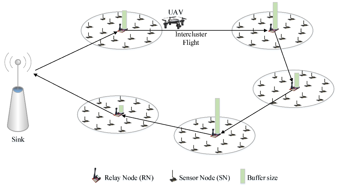
2.1. System Assumptions We consider a remote sensing system that satisfies the following assumptions: (A1) The system includes a wireless sensor network with predetermined cluster heads. Each sensor in the field transmits its information (either directly or indirectly) to one of the cluster heads. (A2) The system also includes a drone that flies on a specific trajectory (to be determined) so that each cluster head transmits its energy to the drone when it is nearby. (A3) The drone’s energy consumption is determined entirely by the length of the drone’s trajectory. (This is the case for example, if the drone flies at a constant velocity, and there is no wind or other conditions that would affect the flight of the drone.) (A4) The drone has a fixed maximum path length, which is determined by the energy capacity of the battery and the rate of energy consumption. (A5) The drone’s location is approximately constant while receiving information from a particular cluster head. This assumption is satisfied in either of the following scenarios: (a) the information transmission from the cluster head occupies only a brief period of time, so that the distance the drone moves during the transmission period is negligible; or (b) the drone slows, hovers, or lands during transmission, and consumes no energy during the transmission period. (A6) The energy expended by the cluster head in information transmission is proportional to the distance between the cluster head and drone raised to a power law exponent. We also consider two alternative criteria for optimization: (O1) Minimize the total energy expended by cluster heads in information transmission. (O2) Minimize the maximum energies expended by cluster heads in information transmission. The choice of suitable optimization criterion will depend on the particular circumstances of the WSN. For example, in a system with many potential alternative cluster heads, then the maximum consumption among cluster heads may be less important than overall power consumption, so criterion O1 may be appropriate. On the other hand, if there are few choices for cluster head, then the cluster head with maximum energy expended will need frequent replacement, so criterion O2 may be a better option. We note that other criteria besides O1 and O2 are possible, with minimal changes to the solution, as we indicate in Section 5. Under assumptions (A1)–(A6) and criteria (O1)–(O2), it follows that an optimum path for the drone will consist of straight-line segments joining the drones’ locations where it harvests energy from the different cluster heads. This conclusion is reflected in the mathematical description in subsequent sections. 2.2. System Parameters and Variables The system parameters include:
  • (xj, yj), j = 1...J: positions of the cluster heads that are sending the information;
  • L: Maximum path length for the drone;
  • p: Power loss exponent.
The system variables include:
  • (uj,vj), j = 1...J : Drone positions for harvesting information from cluster heads. Here, the order of points the drone takes is assumed to be (uj,vj) to (uj+1,vj+1) for j = 1 ...J − 1.
  • (u0,v0), (uJ+1,vJ+1): Drone starting and ending position, respectively.
2.3. Mathematical Formulation of the Optimization Problem Information transmission from cluster head (xj, yj) takes place when the drone is at position (uj, vj). The total energy consumption required for information transfer is the sum of the energies from the J cluster heads, which following assumption (
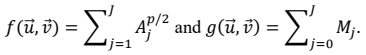
A6), can be represented as a function $$f(\vec{u},\vec{v}){:}$$
```latexf(\vec{u},\vec{v})=\sum_{j=1}^J\left(\left(x_j-u_j\right)^2+\left(y_j-v_j\right)^2\right)^{p/2},```
where $$\vec{u}:=\begin{bmatrix}u_1,....u_J\end{bmatrix}$$ and $$\vec{v}:=\begin{bmatrix}v_1,....v_J\end{bmatrix}$$. 
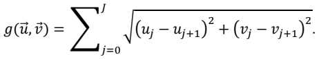
The distance the drone travels is given by $$g(\vec{u},\vec{v})$$, where
The drone’s limited range imposes the constraint $$g(\vec{u},\vec{v})$$ ≤ L, where L is the maximum distance the drone can travel. In the case where L is large enough so that the drone is capable of making a complete tour of the cluster heads, then any such complete tour will give $$g(\vec{u},\vec{v})$$ = 0 and is thus an optimal solution to the problem. So we consider instead the more difficult problem where L is smaller than the smallest tour distance, so $$g(\vec{u},\vec{v})$$ = 0 is impossible. In this case, we may replace the inequality with an equality constraint. This can be seen as follows. Suppose a drone path includes the point (uj, vj) where $$|(u_j,v_j)-(x_j,y_j)|>0.$$ For simplicity, we define:
```latex\vec{w}_{j}{:}=\vec{w}_{j}\big(u_{j},v_{j}\big)\,and\,\vec{z}_{J}{:}=\big(x_{j},y_{j}\big).```
Then, for any δ with 0 < δ ≤ 1, we have
```latex\left|\vec{w}_j+\delta\big(\vec{z}_j-\vec{w}_j\big)-\vec{z}_j\right|=(1-\delta)\big|\vec{w}_j-\vec{z}_j\big|<\big|\vec{w}_j-\vec{z}_j\big|,```
so replacing $$\vec{w}_{j}$$ with $$\vec{w}_{j}+\delta(\vec{z}_{j}-\vec{w}_{j})$$ will reduce the energy function (1). Now, if the drone path length is less than L, then δ > 0 can be chosen sufficiently small such that replacing $$\vec{w}_{j}$$ with $$\vec{w}_{j}+\delta(\vec{z}_{j}-\vec{w}_{j})$$ still yields total drone path length of less than L. Thus, any drone path with a length less than L can be improved—so no drone path with a length less than L can be optimal. We may now formulate the optimization problem. In case (O1), we have
```latex\text{Minimize }f(\vec{u},\vec{v})\text{subject to }g(\vec{u},\vec{v})=L.```
In case (O2), minimizing the maximum transmission energy is equivalent to minimizing $$|\vec{w}_{j}-\vec{z}_{j}|$$ over all j. Using the equality
```latex\lim_{p\to\infty}\bigl(a_{1}^{p}+\cdots+a_{J}^{p}\bigr)^{1/p}=\max_{j}a_{j}\quad if \,a_{j}>0\,\forall \,j,```
with $$a_{j}:=|\vec{w}_{j}-\vec{z}_{j}|$$, we conclude that by taking p sufficiently large, we can approach the solution to (O2) with arbitrary precision. 2.4. Local Optimization Conditions The minimization problem (5) leads to the following Lagrange multiplier condition for a local minimum:
```latex\nabla f(\vec{u},\vec{v})=\lambda\nabla(g(\vec{u},\vec{v})-L),```
where ∇h denotes the gradient of h with respect to $$(\vec{u},\vec{v})$$:
```latex\nabla h(\vec{u},\vec{v}){:}=\left(\frac{\partial f}{\partial u_{1}},...\frac{\partial f}{\partial u_{j}},\frac{\partial f}{\partial v_{1}},...\frac{\partial f}{\partial v_{j}}\right),```
and λ is a Lagrange multiplier. 
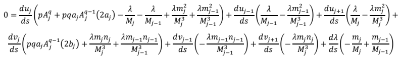
Writing the vector Equation (7) out in terms of components, we have:
```latex\frac{\partial f}{\partial u_{j}}=\lambda\frac{\partial g}{\partial u_{j}};\frac{\partial f}{\partial v_{j}}=\lambda\frac{\partial g}{\partial v_{j}},\quad(j=1\ldots J)```
For notational simplicity, we define new variables. For j = 1….J, let
```latexa_j:=u_j-x_j;b_j:=v_j-y_j;A_j:=a_j^2+b_j^2,```
```latexm_j:=u_j-u_{j+1};n_j:=v_j-v_{j+1};M_j:=\left(m_j^2+n_j^2\right)^{\frac{1}{2}}.```
Then we have:
Using this notation, we have:
```latex\frac{\partial f}{\partial u_{j}}=\frac{\partial f}{\partial A_{j}}\times\frac{\partial A_{j}}{\partial a_{j}}\times\frac{\partial a_{j}}{\partial u_{j}}=(\left(\frac{p}{2}\right)A_{j}^{\frac{p}{2}-1}\times2a_{j}=pa_{j}A_{j}^{q}```
where $$q{:}=\frac{p}{2}-1$$, and
```latex\frac{\partial g}{\partial u_{j}}=\frac{\partial g}{\partial M_{j-1}}\times\frac{\partial M_{j-1}}{\partial m_{j-1}}\times\frac{\partial m_{j-1}}{\partial u_{j}}+\frac{\partial g}{\partial M_{j}}\times\frac{\partial M_{j}}{\partial m_{j}}\times\frac{\partial m_{j}}{\partial u_{j}}=\\\left(\frac12\right)M_{j-1}^{-1}\big(2m_{j-1}\big)(-1)+\bigg(\frac12\bigg)M_j^{-1}\big(2m_j\big)=\frac{m_j}{M_j}-\frac{m_{j-1}}{M_{j-1}}.```
Similarly, we have:
```latex\frac{\partial f}{\partial v_{j}}=pb_{j}A_{j}^{q};\frac{\partial g}{\partial v_{j}}=\frac{n_{j}}{M_{j}}-\frac{n_{j-1}}{M_{j-1}}.```
It follows that we may rewrite the equations in (9) as:
```latexpa_{j}A_{j}^{q}=\lambda\left(\frac{m_{j}}{M_{j}}-\frac{m_{j-1}}{M_{j-1}}\right);pb_{j}A_{j}^{q}=\lambda\left(\frac{n_{j}}{M_{j}}-\frac{n_{j-1}}{M_{j-1}}\right)\quad(j=1\ldots J).```
Equations (16) are required for local optimality and are necessary for global optimality but not sufficient. Thus, the solutions that we provide in this paper may not be optimal for all global situations. We return to this issue in Section 2.8. 2.5. Homotopy Approach to Local Optimization for a Given Path Length Solutions of the fundamental optimization problem (5) for different values of L correspond to solutions of (16) with different values of λ. As L is varied continuously, the value of λ will also vary continuously, and the components of $$\vec{u}$$ and $$\vec{v}$$ will vary continuously as well. This suggests that if we have a solution to (5) for a given value of L, we may be able to perturb that solution differentially to obtain solutions for different values of L. In fact, we do have a solution for a particular value of L: namely f( $$\vec{u}$$, $$\vec{v}$$) = 0 when uj = xj and vj = yj, which solves the constraint $$g(\vec{u},\vec{v})$$ = L when L is equal to the length of the tour that connects the points $$({\vec{x}}_{j},{\vec{y}}_{j})$$ in consecutive order. The smallest value of L for this type of solution occurs when the points $$({\vec{x}}_{j},{\vec{y}}_{j})$$ are ordered so that $$(u_{0},v_{0}),(x_{1},y_{1}),(x_{2},y_{2}),...(x_{J},y_{J}),(u_{J+1},v_{J+1})$$ forms a “travelling salesman” tour that connects all points $$({\vec{x}}_{j},{\vec{y}}_{j})$$ with the smallest possible total length. In practice, we want to find solutions corresponding to L values that are smaller than the length of a full tour. So we start with the full tour and successively “nudge” the solutions so they correspond to smaller and smaller values of L. This is an example of a homotopy approach: start with a solution that is optimal for a different set of conditions and generate a smooth curve of solutions that joins this solution to a solution that satisfies desired conditions. In practice, this smooth curve of solutions is often specified parametrically as the solution to a set of ordinary differential equations. In the next section, we will derive differential equations that can be used to find the parametrized curve that leads to our desired optimal solution. 2.6. Derivation of Differential Equations for Parametrized Homotopy Curve First, we parametrize solutions to (16) using the parameter s, so that aj, bj, Aj, mj, Mj, and λ are all functions of s. As s changes, the equalities cannot change, so we have
```latexp\frac{d}{ds}\big(a_{j}A_{j}^{q}\big)=\frac{d}{ds}\bigg(\lambda\frac{m_{j}}{M_{j}}-\lambda\frac{m_{j-1}}{M_{j-1}}\bigg),\\p\frac{d}{ds}\big(b_{j}A_{j}^{q}\big)=\frac{d}{ds}\bigg(\lambda\frac{n_{j}}{M_{j}}-\lambda\frac{n_{j-1}}{M_{j-1}}\bigg).```
Since we want to find solutions for smaller values of L, we want to ensure that L decreases as s increases. We may ensure this by adding the condition:
```latex\frac{dg}{ds}=-1\Rightarrow\sum_{j=0}^J\frac{dM_j}{ds}=-1.```
Recall that the variables aj, bj, Aj, mj, Mj, in (17) are all functions of $$\vec{u}$$ and $$\vec{v}$$, so the derivatives in (17) can all be expressed in terms of the derivatives $$\frac{du_{j}}{ds}$$ and $$\frac{dv_{j}}{ds}$$ for j = 1,…..J. As a result, we obtain a system of 2J + 1 differential equations for the variables {uj,vj},j = 1….J and λ. We may rewrite the first equation in (17) as (j = 1….J):
```latex0=pA_{j}^{q}\frac{da_{j}}{ds}+pqa_{j}A_{j}^{q-1}\frac{dA_{j}}{ds}-\frac{\lambda}{M_{j}}\frac{dm_{j}}{ds}+\frac{\lambda}{M_{j-1}}\frac{dm_{j-1}}{ds}+\\\frac{\lambda m_{j}}{M_{j}^{2}}\frac{dM_{j}}{ds}-\frac{\lambda m_{j-1}}{M_{j-1}^{2}}\frac{dM_{j-1}}{ds}-\frac{m_{j}}{M_{j}}\frac{d\lambda}{ds}+\frac{m_{j-1}}{M_{j-1}}\frac{d\lambda}{ds}```
The derivatives in (19) may be expressed in terms of { $$\frac{du_k}{ds}$$} and { $$\frac{dv_j}{ds}$$} using the formulas (j = 0…..J):
```latex\begin{gathered}\frac{da_{j}}{ds}=\frac{du_{j}}{ds}; \\\frac{dA_{j}}{ds}=2a_{j}\frac{du_{j}}{ds}+2b_{j}\frac{dv_{j}}{ds}; \\\frac{dm_{j}}{ds}=\frac{du_{j}}{ds}-\frac{du_{j+1}}{ds}; \\\frac{dM_{j}}{ds}=M_{j}^{-1}\left(m_{j}\left(\frac{du_{j}}{ds}-\frac{du_{j+1}}{ds}\right)+n_{j}\left(\frac{dv_{j}}{ds}-\frac{dv_{j+1}}{ds}\right)\right) \end{gathered}```
It follows that (19) with index j will depend on the derivatives $$\frac{du_k}{ds}$$, $$\frac{dv_k}{ds}$$ and $$\frac{dλ}{ds}$$ for k = j $$-$$ 1,j,j + 1 (noting that $${\frac{du_{0}}{ds}}={\frac{dv_{0}}{ds}}={\frac{du_{j+1}}{ds}}={\frac{dv_{j+1}}{ds}}=0$$. By collecting terms corresponding to each derivative, we find (j = 1…..J)
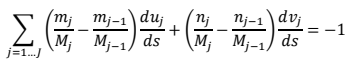
Using various algebraic manipulations and the fact that:
```latex1-\frac{m_j^2}{M_j^2}=\frac{n_j^2}{M_j^2}```
The Equations (19) may be simplified to:
```latex\begin{gathered} 0=\frac{du_{j}}{ds}\left(pA_{j}^{q}\left(1+\frac{2qa_{j}^{2}}{A_{j}}\right)-\frac{\lambda n_{j-1}^{2}}{M_{j-1}^{3}}\right)-\frac{\lambda n_{j}^{2}}{M_{j}^{3}} \\+\frac{du_{j-1}}{ds}\biggl(\frac{\lambda n_{j-1}^{2}}{M_{j-1}^{3}}\biggr)+\frac{du_{j+1}}{ds}\biggl(\frac{\lambda n_{j}^{2}}{M_{j}63}\biggr) \\+\frac{dv_{j}}{ds}(2pqa_{j}b_{j}A_{j}^{q-1}+\frac{\lambda m_{j-1}n_{j-1}}{M_{j-1}^{3}}+\frac{\lambda m_{j}n_{j}}{M_{j}^{3}}) \\-\frac{dv_{j-1}}{ds}\biggl(\frac{\lambda m_{j-1}n_{j-1}}{M_{j-1}^{3}}\biggr)-\frac{dv_{j+1}}{ds}\biggl(\frac{\lambda m_{j}n_{j}}{M_{j}^{3}}\biggr) \\+\frac{d\lambda}{ds}\biggl(-\frac{m_{j}}{M_{j}}+\frac{m_{j-1}}{M_{j-1}}\biggr),j=1\ldots J \end{gathered}```
The J equations associated with the second equation in (17) may be obtained from (23) by exchanging $$u_{k}\leftrightarrow v_{k}$$, $$a_{k}\leftrightarrow b_{k}$$, and $$m_{k}\leftrightarrow n_{k}$$. Finally, (18) can be expressed in terms of derivatives of {uj,vj} as:
The entire system of 2
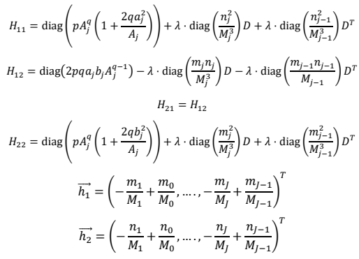
J +1 equations can be represented in matrix form as:
```latexH\frac{d\mathbf{u}}{ds}=z\Rightarrow\frac{d\mathbf{u}}{ds}=H^{-1}\vec{z}```
where H is a (2J + 1) × (2J + 1) matrix, and u,z are column vectors of length 2J + 1, given by the formulas:
```latex\mathbf{u}:=[\vec{u},\vec{v},\lambda]^{T};\\\mathbf{z}:=[0,....0,-1]^{T}```
(i.e., z has a single nonzero entry of −1 in the last component). The matrix H can be decomposed into blocks:
```latexH=\begin{bmatrix}H_{11}&H_{12}&\overrightarrow{h_1}\\H_{21}&H_{22}&\overrightarrow{h_2}\\\overrightarrow{h_1^T}&\overrightarrow{h_2^T}&0\end{bmatrix}```
The blocks Hij can be expressed in terms of diagonal and subdiagonal matrices. First, we introduce some abbreviated notations. Let diag(cj) denote the J × J diagonal matrix with entries c1,...cJ on the diagonal; and let D denote the discrete forward derivative matrix with −1’s on the diagonal and 1’s on the first superdiagonal. Then we have:
2.7. Initial Conditions for Differential Equation In Section 2.5, we suggested that by starting with a complete tour by the drone that visits all sensors and “nudging” the drone’s path, we can find optimal solutions for shorter and shorter path lengths. Unfortunately, the matrix H in (25) is singular when $$(u_{j},v_{j})=(x_{j},y_{j}),j=1....J$$, which corresponds exactly to the case of a complete tour. So, we cannot use this solution as an initial condition. Fortunately, we can address this problem by choosing a solution where the (uj, vj) is slightly offset from (xj, yj) for all j, i.e.,
```latex\begin{pmatrix}u_j,v_j\end{pmatrix}=\begin{pmatrix}x_j,y_j\end{pmatrix}+\vec{\epsilon}_j.```
We need to choose the { $$\vec{\epsilon}_{J}$$ } in such a way that the Lagrange multiplier conditions (7) are satisfied. We also need to choose { $$\vec{\epsilon}_{J}$$} such that the path joining the {(uj, vj)} is smaller than the full tour. The gradient of f($$\vec{u},\vec{v}$$) evaluated at the point for the initial point given by (29) is given by:
```latex\begin{gathered}\nabla f(u_{j},v_{j})=p\left(\left(x_{j}-u_{j}\right)^{2}+\left(y_{j}-v_{j}\right)^{2}\right)\left[(x_{j}-u_{j}),\left(y_{j}-v_{j}\right)\right] \\=p\big|\overrightarrow{\epsilon}_{j}\big|^{p-2}\overrightarrow{\epsilon}_{j} \\=p\big|\overrightarrow{\epsilon}_{j}\big|^{p-1}\widehat{\epsilon}_{j} \end{gathered}```
where $$\widehat{\epsilon}_{J}$$ is the unit vector in the direction of $$\vec{\epsilon}$$. The Lagrange multiplier condition (7) gives:
```latexp\big|\vec{\epsilon}_{j}\big|^{p-1}\widehat{\epsilon}_{j}=\lambda\nabla_{j}g(\vec{u},\vec{v}),```
where
```latex\nabla_{j}g(\vec{u},\vec{v}):=(\frac{\partial g}{\partial u_{j}},\frac{\partial g}{\partial v_{j}})```
Since $$g(\vec{u},\vec{v})$$ is smooth in the vicinity of $$(\vec{u},\vec{v})\approx(\vec{x},\vec{y})$$, we may approximate:
```latex\nabla_{j}g(\vec{u},\vec{v})\approx\nabla_{j}g(\vec{u},\vec{v})|_{\vec{u}=\vec{x}},```
Which may be evaluated using (14) and (15). Denoting the right-hand side of (33) as $$\vec{g_{J}}$$, we have from (31)
```latexp\left|\overrightarrow{\epsilon_{j}}\right|^{p-1}\widehat{\epsilon_{j}}=\lambda\overrightarrow{g_{j}}\\\Rightarrow\widehat{\epsilon_{J}}=\pm\widehat{g_{J}}\mathrm{~and}\left|\epsilon_{j}\right|=\left|\frac{\lambda}{p}\right|^{(\frac{1}{p-1})}\left|\overline{g_{J}}\right|^{(\frac{1}{p-1})}```
Since we are interested in solutions for which g is reduced, we choose the negative sign in (34). Then $$\vec{\epsilon}_{J}$$ is uniquely determined by the values of $$\vec{g_{J}}$$ and λ. By choosing a small value of λ, we may obtain initial values for $$(\vec{u},\vec{v})$$ that are very close to $$(\vec{x},\vec{y})$$, so that the approximation in (33) holds a very high degree of accuracy. In this way, we obtain initial conditions for our differential Equation (25) for which H is not singular and can then apply standard numerical methods for solution. 2.8. Global Optimality for Sufficiently Long Drone Ranges In Section 2.4, we posed the local optimality condition (7) from which the vector differential Equation (25) is derived. To show that a locally optimal solution is globally optimal, we would need to show that it improves over all other locally optimal solutions. We may establish this for the solutions described in Sections 2.5–2.7 for drone ranges that are less than but close to the travelling salesman tour length as follows. Here we give a brief outline of the proof; a more extended presentation is given in Appendix B. Every local optimal solution for a given drone path length will be part of a homotopy of solutions that may be parametrized by path length. As path length increases in the homotopy, the energy consumption decreases until a minimum energy consumption is reached for the entire homotopy. This minimum energy is necessarily nonnegative—and if it is 0, then the homotopy must terminate at a tour that joins all of the cluster heads. The shortest cluster head tour (i.e., the travelling salesman solution) will be the unique optimum in the case when the drone path length is equal to this shortest tour. It follows that for sufficiently long drone path lengths, the solution that belongs to the homotopy that includes the travelling salesman solution will be the unique global optimum. This justifies our claim that the solution of (5) calculated using the homotopy approach outlined in Sections 2.5–2.7 is optimal for sufficiently long drone ranges. The limited nature of this proof does not necessarily mean that the solution we have presented is not globally optimal for shorter drone ranges: global optimality is notoriously difficult to establish rigorously, except in the case where the function to be optimized has nice properties such as convexity. Nonetheless, the proof adds credibility to the expectation that the obtained solution has a strong likelihood of being not just locally optimal but also globally optimal. 2.9. Implementation in Python As described above, the algorithm has two phases. First, an initial ordering of cluster heads is determined, such that the length of a tour joining the cluster heads in this order is minimized among all possible orderings. Once the ordering is set, the homotopy of solutions is computed using the initial conditions and system of differential equations described in Sections 2.7 and 2.5. The final path with the desired path length is selected from the homotopy. For the first phase, the shortest tour joining cluster heads is found using the travelling salesman algorithm as implemented in the python-tsp package. This gives a set of ordered cluster head points, that is, (xj,yj) re-arranged appropriately. For the second phase, the homotopy solution is computed according to the following steps: Step 0: Initialize cluster head locations, initial value of λ, and step size h (typically on the order of 0.1), Step 1: Find a minimal initial path joining the cluster head points using a travelling salesman algorithm. Step 2: Determine the initial points of the closest approach to be a small distance away from the cluster head points, according to the algorithm described in Section 2.7. Step 3: Solve the homotopy Equations (25) numerically. Initially, we used the odeint solver from the scipy package but encountered instabilities when the path vertices began to merge. We succeeded better using a Runge Kutta-4 code obtained from the web and modified for our purpose. Appendix A gives a more detailed description of the code as well as a link to a Github page where the code can be downloaded. 
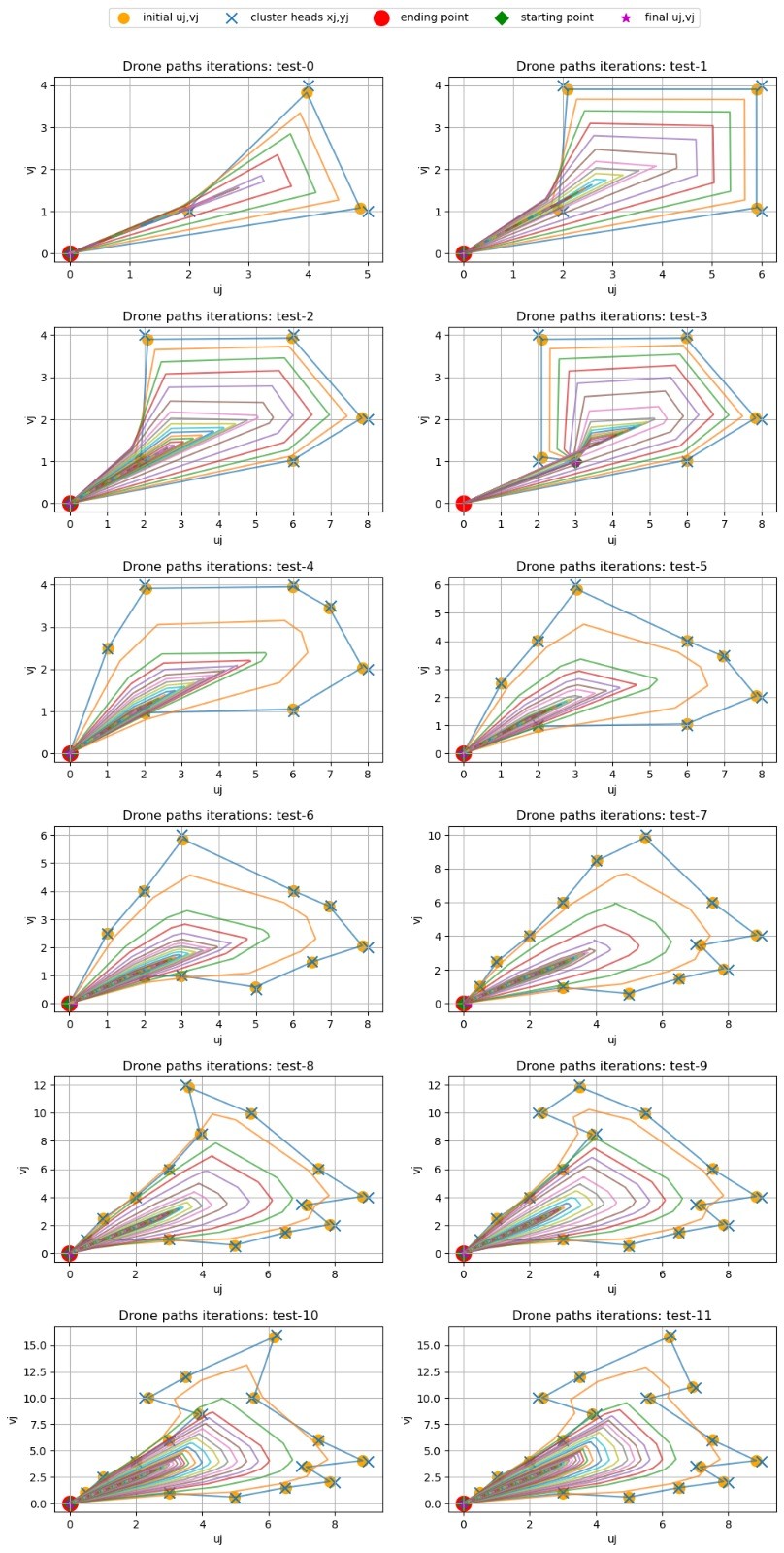
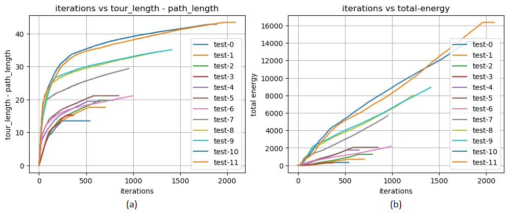
2.10. Specification of Test Cases The Python implementation of the algorithm was tested by simulating a number of different cluster head configurations, with various numbers of cluster heads and drone starting positions. The test configurations used have the following cluster head position: Case 1: [(2, 1), (2, 4), (6, 4), (6, 1)] Case 2: [(2, 1), (2, 4), (8, 2), (6, 4), (6, 1)] Case 3: [(2, 1), (2, 4), (8, 2), (6, 4), (6, 1)] Case 4: [(2, 1), (2, 4), (8, 2), (6, 4), (6, 1), (7, 3.5), (1, 2.5)] Case 5: [(2,1), (2, 4), (8, 2), (6, 4), (6, 1), (7, 3.5), (1, 2.5), (3,6)] Case 6: [(2,1), (2, 4), (8, 2), (6, 4), (6.5, 1.5), (7, 3.5), (1, 2.5), (3,6), (3,1), (5,0.5)] Case 7: [(0.5,1), (2, 4), (8, 2), (9, 4), (6.5, 1.5), (7, 3.5), (1, 2.5), (3,6), (3,1), (5,0.5),(7.5,6), (4,8.5), (5.5,10)] Case 8: [(0.5,1), (2, 4), (8, 2), (9, 4), (6.5, 1.5), (7, 3.5), (1, 2.5), (3,6), (3,1), (5,0.5),(7.5,6), (4,8.5), (5.5,10), (3.5,12)] Case 9: [(0.5,1), (2, 4), (8, 2), (9, 4), (6.5, 1.5), (7, 3.5), (1, 2.5), (3,6), (3,1), (5,0.5),(7.5,6), (4,8.5), (5.5,10), (3.5,12), (2.25,10)] Case 10: [(0.5,1), (2, 4), (8, 2), (9, 4), (6.5, 1.5), (7, 3.5), (1, 2.5), (3,6), (3,1), (5,0.5),(7.5,6), (4,8.5), (5.5,10), (3.5,12), (2.25,10), (6.25,16)] Case 11: [(0.5,1), (2, 4), (8, 2), (9, 4), (6.5, 1.5), (7, 3.5), (1, 2.5), (3,6), (3,1), (5,0.5),(7.5,6), (4,8.5), (5.5,10), (3.5,12), (2.25,10), (6.25,16), (7,11)] 
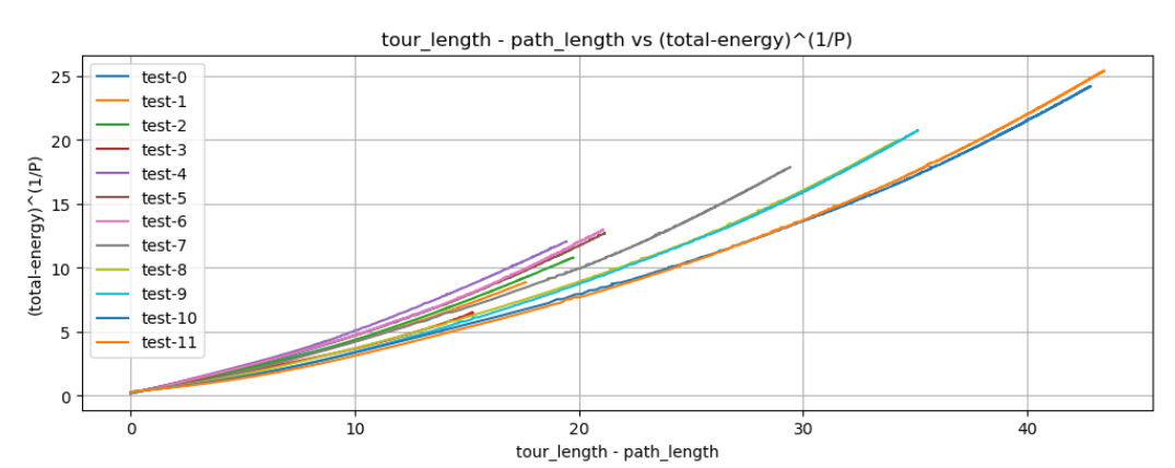
These configurations were chosen manually so as to have homotopy solutions that are easily visible as well as to be sufficiently similar so that trends in the homotopy as the number of points increases are also visible. All cases used a transmission power loss exponent of 2, with the finishing position of drone equal to (0,0). The drone path starting point is (0,0), except for Case 3 in which the starting point is (3,1). For each configuration, the travelling salesman tour was computed, as well as the homotopy of solutions obtained when the drone path length L is decreased from the travelling salesman tour length down to the minimum path joining the tour starting and ending point. A step size of 0.1 was used for the numerical solution for all cases.

3. Results

Figure 2, Figure 3 and Figure 4 display results from simulations of the test cases described in Section 2.10 using the Python code described in Appendix A. Figure 2 contains a 6 × 2 grid of plots that shows results from the test scenarios listed above. Each plot shows solutions in the homotopy corresponding to different drone path lengths. The longest path in each homotopy is the travelling-salesman path that joins the cluster heads; while the shortest is the straight-line path that joins starting and ending points. The algorithm computes the vertices from longest path to shortest, according to the ODE in equation (25) with initial conditions $$(\vec{u},\vec{v})=(\vec{x},\vec{y})$$, where the (xj,yj ) are in travelling salesman order. Initially, the paths roughly preserve the original shape as they shrink (in fact, it can be shown that as the path shrinks, the path vertices always move in the direction of the angle bisectors of the path polygon.) After several iterations, path vertices merge: for example, the first figure in the first row starts with a path containing 5 segments, which eventually becomes 4 and then 3 segments as the path length shrinks. Similar changes occur in the other figures. The left-hand graph in Figure 3 plots the difference between the travelling salesman tour length and the length of the drone’s path (which for simplicity, we denote as the “path defect”) as a function of the iteration number in the ODE solution, for each of the test cases. The initial path length is equal to the tour length; hence, all graphs start from (0,0). The path defect increases more rapidly for scenarios with more cluster heads and longer travelling salesman tour lengths. For all scenarios, the rate of increase of path defect slows as the number of iterations increases. Eventually, the curves become flat when the homotopy reaches the minimum path that joins (u0,v0 ) and (uJ+1,vJ+1). The right-hand graph in Figure 3 shows the WSN’s energy expenditure as a function of step number. As expected, this increases with iteration number as the path length decreases. There are noticeable bends in both graphs, which occur at the same iteration number. For example, in the curves for test-7, test-8 and test-9 there are concurrent bends in both the defect curve and the total energy curve, which occur near iteration numbers 75, 125, and 150, respectively. In the homotopy, the bend indicates the merger of two path vertices so that two cluster heads both correspond to a single vertex. This shows that vertex mergers slow down the algorithm’s progress. The tradeoff between drone path length and energy expenditure is more clearly shown in Figure 4, which plots the p’th root of cluster head energy consumption on the vertical axis versus cluster head tour length minus drone path length on the horizontal axis. In our simulations p = 2, so the p’th root of energy is the ℓ2 norm of the vector $$[|\vec{z}_{1}-\vec{w}_{1}|,\ldots,|\vec{z}_{J}-\vec{w}_{J}|]$$ consisting of distances between cluster heads and corresponding drone path vertices. In the case where all distances $$|\vec{z}_{j}-\vec{w}_{j}|$$ are approximately equal, then the 2 norm is nearly proportional to the mean distance between the cluster head and the corresponding drone vertex. The linear section of the graphs in Figure 4 indicates an initial linear dependence of the distance between cluster heads and drone vertices as the path defect increases. However, as the path defect increases (corresponding to a decrease in drone range), the dependence of total energy on path length becomes noticeably convex. Unlike the energy versus iteration and path defect versus iteration curves in Figure 3, there are no bends in these curves. This indicates that the bends reflect convergence issues for the numerical solution for the homotopy rather than a change in the trends in energy over the homotopy as the drone range is varied. Figure 5 represents different runtime characteristics associated with the numerical solution of equation (15) for different numbers of cluster heads and different drone ranges. The three panels in Figure 5 represent the total runtime, number of Runge-Kutta iterations, and runtime per iteration for the 12 scenarios shown in Figure 2 for four different drone ranges, plotted as a function of the number of vertices in the solution path. For each of the 12 scenarios, we chose four evenly-spaced drone ranges of 0.2, 0.4, 0.6, and 0.8 times the minimum range required to reduce the objective function $$f(\vec{u},\vec{v})$$ to 0, which is equal to the length of the travelling salesman path joining the points {(xj,yj)}. The graphs show gradual increases in runtime as the number of cluster heads increases. The runtime per iteration does increase for more cluster heads (as expected, since more variables must be solved for), but this increase is offset by a concurrent general decrease in the number of iterations required for each drone range. Although the full algorithm requires the initial solution of a travelling salesman problem in addition to the solution of (15), we do not include the runtimes for the travelling salesman problem in Figure 5. It is well known that an exact solution depends exponentially on the number of vertices. However, there are many algorithms with lower complexity (including both stochastic and heuristic algorithms) that can be used to obtain near-optimal tours.
Figure 2. Drone path homotopy solutions for 1 different test scenarios. The cluster head positions are indicated by X’s. The different colored lines are drone path solutions for different values of maximum drone range, with the drone start and end points as indicated.
Figure 3. (<b>a</b>) Path defect (defined as the length of a tour of the cluster heads minus the length of the drone path) plotted as a function of number of iterations in the numerical solution of the matrix differential Equation (25). (<b>b</b>) Total energy expended by sensors for a single tour, as a function of iteration number. Both graphs show results for 2000 iterations for the 12 test scenarios shown in Figure 2.
Figure 4. (total energy)<sup>1/P</sup> plotted as a function of path defect (defined as the TSP tour length minus the drone path length) for the 12 scenarios shown in Figure 2.
Figure 5. (<b>a</b>) Run times for the Runge-Kutta ODE for the 12 scenarios shown in Figure 2, plotted as a function of the number of cluster heads (equal to the number of path vertices), for different drone ranges. The drone range for each scenario is specified as a fraction of the length of the travelling salesman path joining the cluster heads. The four curves correspond to drone ranges equal to 20%, 40%, 60%, and 80% of the travelling salesman path (longer drone ranges take less time to compute). (<b>b</b>) Number of iterations (with step size <i>h</i> = 0.1) required for the Runge-Kutta algorithm to compute solutions with the specified drone ranges. (<b>c</b>) Execution time per iteration for the same set of solutions as the other two graphs. All simulations were performed using Google Colab.

4. Conclusions

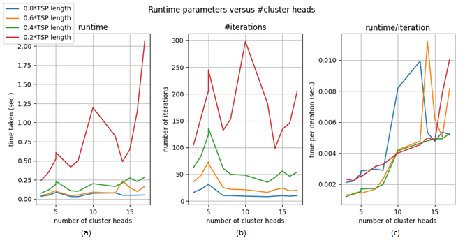
The solution described above for finding optimal drone information-harvesting paths is locally and globally optimal for sufficiently long drone ranges. The numerical solution algorithm executes quickly enough that it can be implemented in real-time, and execution time grows slowly with the size of the system. The solution can be used either to optimize total transmit power consumption and maximum power consumption by cluster heads. However, there are limitations in that the speed of execution slows considerably when the drone range decreases below a certain point (i.e., when path vertices begin to merge), and global optimality for comparatively short drone ranges is uncertain.

5. Future Work

The following future work is proposed in order to improve upon this research.
  • The proposed algorithm supposes that the cluster head positions are predetermined. Alternatively, it is possible to use the algorithm as a component in a more comprehensive algorithm that does co-optimization of cluster head positions and drone path in systems where alternative cluster heads are a possibility.
  • Equation (5) does not take into account various environmental factors such as obstacles or wind speed. It is also not robust to possible sensor node failures. The equation would need to be elaborated to include terms that reflect these factors. Also, the equations are limited to optimization criteria O1 and O2. Different optimization criteria can be accommodated by modifying the Equation (1) for the function $$f(\vec{u},\vec{v})$$, which then requires recalculation of the partial derivatives $$\frac{\partial f}{\partial u_{j}}$$ and $$\frac{\partial f}{\partial v_{j}}$$ which appear in Equations (9) and following.
  • The numerical homotopy solution code has not been fully optimized to decrease execution times. In particular, existing solver packages and/or variable step-size solution algorithms may be explored. In addition, we have remarked that the algorithms slow down after drone path vertex mergers. Future work may explore ways to avoid this slowdown. One possibility is to modify the algorithm so that when path vertices merge, the two associated cluster heads may be replaced by a single virtual cluster head that produces the same power loss. Then, the homotopy solution can be continued with vectors $$\vec{u}$$, $$\vec{v}$$ that each have one less component.
  • The algorithm can be modified to accommodate moving cluster heads, by expressing $$\vec{x}$$,$$\vec{y}$$,$$\vec{u}$$, and $$\vec{v}$$ as functions of time t, and then inverting the time dependence of $$\vec{u}$$ and $$\vec{v}$$ to obtain $$\vec{x}$$ and $$\vec{y}$$ as functions of $$\vec{u}$$ and $$\vec{v}$$. Then the same homotopy approach can be used with modified equations for the derivatives of $$\left\{a_{j}\right\}_{j=1...J}$$ and $$\{b\}_{j=1...J}$$ in (13) and following.
  • Further explorations of the question of global optimality may be pursued. As the proof in Appendix B shows, any globally optimal solution must be part of a homotopy that includes some ordering of the cluster head points. It follows that in some cases, better solutions may be found by computing homotopies for different orderings of the cluster heads.

Appendix A. Python Implementation

Appendix A.1. Link to Code The Python code used to generate the figures shown in Section 3 is available at: https://github.com/ganap-ram/drone. Appendix A.2. Implemented Equations This section describes the differential equations used to solve as implemented in the Python code. Although the implementation is mathematically equivalent to the description in Section 2.5, the notation used is somewhat different. For notational and coding simplicity, we define some intermediate variables:
```latexu_{j},v_{j}=j^{th}\mathrm{turning~point~of~drone~j=1~...J}\\a_{j}=u_{j}-x_{j}\\b_{j}=v_{j}-y_{j}\\A_{j}=a_{j}^{2}+b_{j}^{2}\\m_{j}=u_{j}-u_{j+1}\\n_{j}=v_{j}-v_{j+1}\\M_{j}=m_{j}^{2}+n_{j}^{2}\\H_{j}=M_{j}^{3/2}\\q=\frac{p}{2}-1\\r=1/2```
The following are the various coefficient values of the derivatives in the matrix:
```latex\begin{gathered}S_{j1}=\lambda\frac{M_{j-1}-m_{j-1}^{2}}{H_{j-1}} \\S_{j2}=-\lambda\frac{m_{j-1}n_{j-1}}{H_{j-1}} \\S_{j3}=2pqa_{j}^{2}A_{j}^{q-1}+pA_{j}^{q-1}-\lambda\frac{H_{j}\Big(M_{j-1}-m_{j-1}^{2}\Big)+H_{j-1}(M_{j}-m_{j}^{2})}{H_{j-1}H_{j}} \\S_{j4}=2pqa_{j}b_{j}A_{j}^{q-1}+\lambda\frac{m_{j-1}n_{j-1}H_{j}+m_{j}n_{j}H_{j-1}}{H_{j-1}H_{j}} \\S_{j5}=\lambda\frac{M_{j}-m_{j}^{2}}{H_{j}} \\S_{j6}=-\lambda\frac{m_{j}n_{j}}{H_{j}} \end{gathered}```
```latex\begin{gathered}w_{j}= \frac{-m_{j-1}\sqrt{M_{j}}+m_{j}\sqrt{M_{j-1}}}{\sqrt{M_{j-1}M_{j}}} \\t_{j1}=-\lambda\frac{m_{j-1}n_{j-1}}{H_{j-1}} \\t_{j2}=\lambda\frac{M_{j-1}-n_{j-1}^{2}}{H_{j-1}} \\t_{j3}=2pqa_{j}b_{j}A_{j}^{q-1}+\lambda\frac{m_{j-1}n_{j-1}H_{j}+m_{j}n_{j}H_{j-1}}{H_{j-1}H_{j}} \\t_{j4}=2pqb_{j}^{2}A_{j}^{q-1}+pA_{j}^{q}-\lambda\frac{H_{j}\big(M_{j-1}-n_{j-1}^{2}\big)+H_{j-1}(M_{j}-n_{j}^{2})}{H_{j-1}H_{j}} \\t_{j5}=-\lambda\frac{m_{j}n_{j}}{H_{j}} \\t_{j6}=\lambda\frac{M_{j}-n_{j}^{2}}{H_{j}} \\z_{j}=\frac{-n_{j-1}\sqrt{M_{j}}+n_{j}\sqrt{M_{j-1}}}{\sqrt{M_{j-1}M_{j}}} \end{gathered}```
And the differential equations have the form (j = 1 . . . J):
```latex\begin{gathered}s_{j1}\frac{du_{j-1}}{ds}+s_{j2}\frac{dv_{j-1}}{ds}+s_{j3}\frac{du_{j}}{ds}+s_{j4}\frac{dv_{j}}{ds}+s_{j5}\frac{du_{j+1}}{ds}+s_{j6}\frac{dv_{j+1}}{ds}-c1\frac{d\lambda}{ds}=0 \\t_{j1}\frac{du_{j-1}}{ds}+t_{j2}\frac{dv_{j-1}}{ds}+t_{j3}\frac{du_{j}}{ds}+t_{j4}\frac{dv_{j}}{ds}+t_{j5}\frac{du_{j+1}}{ds}+t_{j6}\frac{dv_{j+1}}{ds}-c2\frac{d\lambda}{ds}=0 \\\frac{dg}{ds}=-1\Rightarrow\sum_{j=1}^{J}\left(\frac{\partial g}{\partial u_{j}}\frac{du_{j}}{ds}+\frac{\partial g}{\partial u_{j}}\frac{dv_{j}}{ds}\right)=-1 \end{gathered}```
This is represented in the matrix notation as:
```latexKD=C```
where:

Appendix B. Mathematical Proof of Global Optimality

In this appendix, we give a more extended presentation of the argument outlined in Section 2.8, which asserts that the homotopy solution found in Sections 2.5–2.7 is a globally optimal solution of (5) for drone ranges that are less than but close to the travelling salesman tour length. A completely rigorous mathematical argument would be tedious to present, but a step-by-step outline is as follows. Suppose first we restrict to drone path solutions such that (uj,vj) is in the same order of (xj,yj ), j = 1,…J where (xj,yj) is the travelling salesman order of cluster heads. Suppose also that $$\left(\vec{u}^{(ts)}(L),\vec{v}^{(ts)}(L)\right)$$ is a globally optimal solution for the drone path satisfying the constraint $$g\big(\vec{u}^{(ts)}(L),\vec{v}^{(ts)}(L)\big)$$ = L. Any globally optimal solution of (5) is also locally optimal: so $$\left(\vec{u}^{(ts)}(L),\vec{v}^{(ts)}(L)\right)$$ is also locally optimal. Then $$\left(\vec{u}^{(ts)}(L),\vec{v}^{(ts)}(L)\right)$$ is part of a homotopy of solutions using the same construction we showed in Sections 2.5–2.7. The homotopy consists of locally optimal solutions $$\left(\vec{u}^{(ts)}(s),\vec{v}^{(ts)}(s)\right)$$ satisfying $$g\big(\vec{u}^{(ts)}(s),\vec{v}^{(ts)}(s)\big)$$ = s, where s can take values in a closed interval containing L. Define the function $$f_{(ts)}(s)=f\big(\vec{u}^{(ts)}(s),\vec{v}^{(ts)}(s)\big)$$. The function f(ts) decreases strictly as s increases, because if the drone path is lengthened, it is always possible to move closer to the cluster heads; and as long as f(ts) (s) is positive, it is always possible to decrease fI by increasing the path length. It follows that the minimum value of f(ts) (s) on the homotopy cannot be positive, so $$\left(\vec{u}^{(ts)}(L),\vec{v}^{(ts)}(L)\right)$$ must be connected by a homotopy to ( $$\vec{x},\vec{y}$$) where the components of $$\vec{x}$$ and $$\vec{y}$$ are in travelling salesman order. So the solution in this homotopy whose length is equal to the travelling salesman tour length of cluster heads (denoted by $$L^{(ts)}$$) corresponds to a value of $$f_{(ts)}\big(L^{(ts)}\big)$$ = 0. Now, we consider solutions where (uj,vj ) receives the information from $$(x_{\sigma(j)},y_{\sigma(j)})$$ where σ is a permutation of (1,…J). By similar arguments as in the previous paragraph, any locally optimal solution corresponding to a path length L is part of a homotopy $$\left(\vec{u}^{(\sigma)}(s),\vec{v}^{(\sigma)}(s)\right)$$ with associated strictly decreasing function $$f_{\sigma}(s):=f\big(\vec{u}_{\sigma}(s),\vec{v}_{\sigma}(s)\big)$$, which includes a solution $$\left(\vec{u}^{(\sigma)}\big(L^{(\sigma)}\big),\vec{v}^{(\sigma)}\big(L^{(\sigma)}\big)\right)$$ for path length $$L^{(\sigma)}>L$$ such that $$f_{\sigma}\big(L^{(\sigma)}\big)=0$$. But this implies that $$\left(\vec{u}^{(\sigma)}\big(L^{(\sigma)}\big)_{j^{\prime}},\vec{v}^{(\sigma)}\big(L^{(\sigma)}\big)_{j}\right)=\big(x_{\sigma(j)},y_{\sigma(j)}\big)$$,j = 1,…J, which in turn implies that $$L^{(\sigma)}$$ is the length of the tour of the points $$\left\{\left(x_{j},y_{j}\right)\right\}_{j=1...J}$$ in the order given by σ. This means that $$L^{(\sigma)}\geq L^{(ts)}$$, and $$L^{(\sigma)}=L^{(ts)}$$ if and only if σ gives a travelling salesman ordering of the nodes in $$\vec{x},\vec{y}$$. Since the function fσ(s) is strictly decreasing, it follows that $$f_\sigma(L^{(ts)})$$ > $$f_{opt}(L^{(ts)}$$ for all permutations σ for which $$(x_{\sigma(j)},y_{\sigma(j)})$$ is not a travelling salesman permutation. Let $$\tilde{f}:=\min_{\sigma\neq I}f_\sigma $$, where the minimum is taken over all non-travelling salesman permutations. Then we also have $$\tilde{f}\big(L^{(ts)}\big)>f_{(ts)}(L^{(ts)})$$. It follows by continuity that there is an $$\tilde{L}$$ with 0 < $$\tilde{L}$$ < $$L^{(ts)}$$ such that $$\tilde{f}(s)>f_{(ts)}(s)$$ for $$\tilde{L}\leq s\leq L$$. In other words, the solution $$\begin{pmatrix}\vec{u}^{(I)}(s),\vec{v}^{(I)}(s)\end{pmatrix}$$ is a local optimum such that $$f\left(\vec{u}^{(I)}(s),\vec{v}^{(I)}(s)\right)$$ is less than the value of f for any other local optimum. It follows that $$\left(\vec{u}^{(ts)}(s),\vec{v}^{(ts)}(s)\right)$$ is a global optimum for $$\tilde{L}$$ < s $$\leq L^{(ts)}$$. Note that this proof does not give a practical, constructive method for finding $$\tilde{L}$$ it only shows that it exists. However, the proof does indicate that any global optimum will be part of some homotopy that includes the points {(xj,yj)},j = 1…J in some order. This fact indicates that other candidate global optimal solutions can be found by creating homotopies starting from other (non-travelling salesman) tours of the cluster heads points.

Acknowledgments

The authors wish to thank Dr. Aristide Tsemo for his thorough review of the equations in Section 2.6, which resulted in several corrections. We also wish to thank the reviewers of this paper, who made several valuable suggestions for improvements.

Author Contributions

Conceptualization, R.G. and C.T.; Methodology, R.G. and C.T.; Software, R.G.; Validation, R.G. and C.T.; Formal Analysis, R.G. and C.T.; Investigation, R.G. and C.T.; Writing—Original Draft Preparation, R.G. and C.T.; Writing—Review & Editing, R.G. and C.T.; Visualization, R.G. and C.T.; Supervision, C.T.

Ethics Statement

Not applicable.

Informed Consent Statement

Not applicable.

Funding

This research received no external funding.

Declaration of Competing Interest

The authors declare that they have no known competing financial interests or personal relationships that could have appeared to influence the work reported in this paper.

References

1.
Nguyen MT, Nguyen CV, Do HT, Hua HT, Tran TA, Nguyen AD, et al. UAV-assisted data collection in wireless sensor networks: A comprehensive survey. Electronics 2021, 10, 2603. [Google Scholar]
2.
Wei Z, Zhu M, Zhang N, Wang L, Zou Y, Meng Z, et al. UAV-assisted data collection for internet of things: A survey. IEEE Int. Things J. 2022, 9, 15460–15483. [Google Scholar]
3.
Memos VA, Psannis KE. UAV-based smart surveillance system over a wireless sensor network. IEEE Commun. Stand. Mag. 2021, 5, 68–73. [Google Scholar]
4.
Qadir Z, Zafar MH, Moosavi SKR, Le KN, Tam VW. Optimizing UAV path for disaster management in smart cities using metaheuristic algorithms. In Computational Intelligence for Unmanned Aerial Vehicles Communication Networks; Springer International Publishing: Cham, Switzerland, 2022; pp. 225–244.
5.
Qadir Z, Zafar MH, Moosavi SKR, Le KN, Mahmud MP. Autonomous UAV path-planning optimization using metaheuristic approach for predisaster assessment. IEEE Int. Things J. 2021, 9, 12505–12514. [Google Scholar]
6.
Dac-Tu H, Esten IG, Tor AJ. Heuristic algorithm and cooperative relay for energy efficient data collection with a UAV and WSN. In Proceedings of the 2013 International Conference on Computing, Management and Telecommunications (ComManTel), Ho Chi Minh City, Vietnam, 21–24 January 2013, pp. 346–351.
7.
Liu S, Wei Z, Guo Z, Yuan X, Feng Z,  Performance analysis of UAVs assisted data collection in wireless sensor network. In Proceedings of the 2018 IEEE 87th Vehicular Technology Conference (VTC Spring), Porto, Portugal, 3–6 June 2018, pp. 1–5.
8.
Gong J, Chang TH, Shen C, Chen X. Flight time minimization of UAV for data collection over wireless sensor networks. IEEE J. Sel. Areas Commun. 2018, 36, 1942–1954. [Google Scholar]
9.
Skiadopoulos K, Giannakis K, Tsipis A, Oikonomou K. Impact of drone route geometry on information collection in wireless sensor networks. Ad. Hoc. Netw. 2020, 106, 102220. [Google Scholar]
10.
Ho DT, Grøtli EI, Sujit PB, Johansen TA, De Sousa JB.Performance evaluation of cooperative relay and Particle Swarm Optimization path planning for UAV and wireless sensor network. In Proceedings of the 2013 IEEE Globecom Workshops (GC Wkshps), Atlanta, GA, USA, 9–13 December 2013, pp. 1403–1408.
11.
Zhu M, Wei Z, Qiu C, Jiang W, Wu H, Feng Z. Joint data collection and sensor positioning in multi-UAV-assisted wireless sensor network. IEEE Sens. J. 2023, 23, 23664–23675. [Google Scholar]
TOP