1. Introduction
Globally, total flood-related financial damages are projected to increase to $52 billion by 2050, up from $6 billion in 2005 [
1]. The total property damage and loss of life due to the 2014 flooding events across the United States were estimated to be almost $3 billion, accounting for 36% of the overall average during the 30-year period from 1984 to 2013 [
2]. A flood risk assessment study for Los Angeles, California indicated that a projected 100-year flood could potentially affect a median of 425,000 people and result in a median economic loss of $56 billion [
3].
Beyond the likelihood of experiencing a flood of a certain magnitude and duration, the extent of financial loss also depends on societal reactions to the event and the levels of societal vulnerability [
4]. The 21st century increases in US flood damage may be attributed to rising societal vulnerability in addition to increases in precipitation and streamflow [
5,
6,
7,
8,
9]. Since flood risk is a product of flood hazard, exposure, and societal vulnerability, measures such as providing more reliable flood quantiles estimate can improve societal resilience and decrease flood risk [
4].
Reliable flood forecasting requires acknowledging nonstationarity in climate as well as nonstationarity due to anthropogenic disturbances such as land use/cover change, water withdrawal, river regulation, and reservoir construction [
10,
11,
12,
13,
14]. To facilitate understanding of the influence of nonstationarity on flood forecasting, it is vital to study both undisturbed and disturbed watersheds [
15,
16]. Disturbed watersheds have experienced anthropogenic disturbances during the flood record period, while undisturbed watersheds have no or minimum disturbances [
17]. Studying reference streamflow gauging stations at undisturbed watersheds along with nonreference stations at disturbed watersheds will improve regional flood frequency analysis and forecasting since the distinction in physiographic characteristics can affect flood quantile estimates [
18,
19,
20,
21].
Several studies on flood analysis across the US have used peak flow data, taking into account differences between reference and nonreference streamflow gauges due to factors such as urbanization or damming, but they did not clearly separate gauges into distinct clusters (e.g., [
12,
22,
23,
24]).
In this study, we considered two clusters of 26 reference and 78 nonreference sites with peak flow records of at least 100 years and no missing data across the contiguous US. We compared the differences between flood quantile estimates at reference sites with those at nonreference sites. We utilized two statistical distributions, Log Pearson Type III (LP3) and Generalized Extreme Value (GEV), to estimate flood quantiles. These robust, resistant, and efficient distributions have been tested extensively (e.g., [
24,
25,
26,
27,
28,
29,
30,
31,
32,
33,
34,
35,
36,
37,
38,
39,
40].
This article aims to: (1) investigate whether the choice of LP3 or GEV distribution is limited by a site being reference or nonreference, and (2) determine the impact of partitioning sites into reference and nonreference on estimating the shape parameters of LP3 and GEV distributions. These objectives were studied throughout the contiguous US using the most recent peak flow data to reassess the design flood information. The results can help engineers and water managers better prepared for changes in flood frequency and magnitude in nonstationary conditions and improve infrastructure design and reservoir management.
2. Materials and Methods
2.1. Data
Peak flow information was obtained from the US Geological Survey’s (USGS) Surface-Water Data for the Nation (https://nwis.waterdata.usgs.gov/usa/nwis/peak). The USGS Hydro-Climatic Data Network (HCDN) (https://on.doi.gov/2wHG9z8) was utilized to screen and select among streamflow gauging stations with minimal or no anthropogenic disturbances, known as reference sites [
41,
42]. Among 9067 USGS gauging stations in the contiguous US [
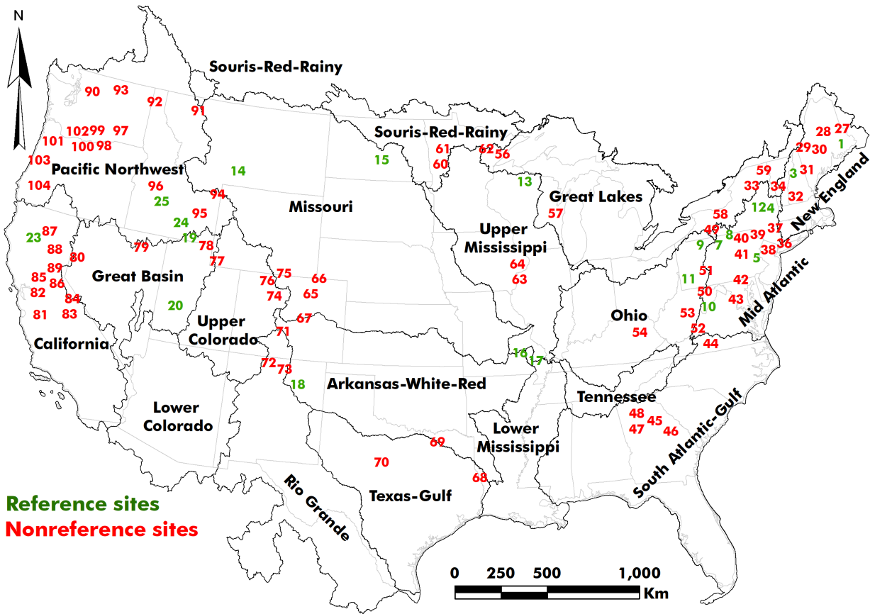
17], we chose 26 reference and 78 nonreference sites with more than 100 years of peak flow information to avoid the uncertainty associated with short-length records (). Additionally, the 18 water-resources regions of the contiguous US (2-digit Hydrologic Unit) are identified on . More characteristics of the study sites are presented in the appendix (Table S1).
. The spatial distribution of 26 reference and 78 nonreference study sites with more than 100 years of peak flow observations across the contiguous United States. The names and boundaries of HUC02 regions were identified [
43].
In this study, we used the LP3 (with product moment parameter estimation) and GEV (with linear moment parameter estimation) distributions, which have been extensively used to estimate flood quantiles throughout the contiguous US. These two distributions are among the most popular and well-accepted statistical distributions recommended for flood frequency analysis [
15,
22,
29,
35,
44]. The product moment estimation of the LP3 parameters is based on three data moments: mean, variance, and skewness. The product moment estimation utilizes higher powers of deviation from the mean; therefore, it is highly sensitive to rare or extreme high flood values [
26].
The product moment estimation of distribution parameters for highly skewed flood flow information can be replaced by linear moment approximation, also known as the L-moment method [
45]. The GEV analysis with L-moment approximation for distribution parameters has been globally applied for both at-site and regional flood frequency analysis [
35,
46,
47,
48,
49]. The GEV produces less biased flood quantile estimations compared to LP3 [
50]. The formulation of LP3 and GEV distributions is detailed in the following section. The authors developed a computational code in R to estimate flood quantiles using the formulations presented for LP3 and GEV distributions.
2.2.1. The LP3 Distribution with Product Moment Parameter Estimation
The LP3 distribution has the following Probability Density Function (PDF) [
50]:
where
X is the natural logarithm of the observed peak flow data, i.e., $$X=\ell n(Q)$$.
The Cumulative Distribution Functions (CDF) for LP3 distribution can be calculated by integrating the PDF from “0” to “x”. However, the integral of the PDF does not have a simple closed-form solution; thus, for practical purposes, the CDF of LP3 distribution is often computed numerically [
50].
At first, the mean ($$\hat{\mu}_{X}$$, first moment), variance ($$\hat{\sigma}_{X}^{2}$$, second moment), and skewness ($$\hat{\gamma}_{X}$$, third moment) of the population were calculated from the peak flow observations. The moments of observations provide an acceptable population estimate. The mean, variance, and skewness of the “
n” observations (shown by subscript
X) were estimated in the following steps:
With the estimated moments, the LP3 distribution parameters of shape ($$\alpha$$), scale ($$\beta$$), and location ($$\xi$$) can be calculated through the following equations [
50]:
The shape, scale, and location parameters are employed to find the mean, variance, and skewness (the moments of distribution, shown by subscript
Q) of the LP3 distribution [
50]:
The moments of distribution were utilized to estimate the peak flow quantiles [
51]:
The Wilson-Hilferty formula provides an acceptable estimate for the frequency factor $$K_{P}(\gamma_{Q})$$ where $$0.01\leq P\leq0.99$$ and $$\left|\gamma\right|< 2$$ [
50,
51]. If the return period is considered as
T , then $$P=1-1/T$$. Depending on
P,
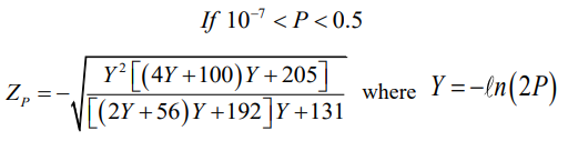
ZP which is the
Pth quantile of the standard normal distribution with mean and variance equal to zero and one, respectively, can be estimated by [
52]:
In order to visually check the goodness-of-fit for LP3, the empirical probability function was used based on the Blom formula [
53]:
where
i is the rank of the observations in which
i = 1 goes with the greatest observation. The probability of occurrence was calculated as:
If LP3 is suitable for flood frequency analysis, then the plot of $$Z_i=\frac{X_i-\hat{\mu}_X}{\hat{\sigma}_X}$$ vs. $$K_{P_i}\begin{pmatrix}\gamma_Q\end{pmatrix}$$ should fall on 1:1 line [
22].
2.2.2. The GEV Distribution with L-Moment Parameter Estimation
GEV was introduced by Jenkinson (1995) [
54]. Wallis (1980) [
55] and Greis and Wood (1981) [
56] further developed its hydrologic application using the index-flood procedure and probability-weighted moments (PWM). The closed-form solution of GEV inverse function enhances its suitability for flood frequency analysis [
27]. The GEV has the corresponding CDF [
50]:
GEV does not require any data transformation. The
X is an ordered series of observations
Q from the largest to the smallest. Let’s assume there are
K sites in the region of interest with peak flow records of $$\begin{bmatrix}X_t(k)\end{bmatrix}$$ where $$t=1,2,...,n_{k}$$ years of information and $$k=1,2,...,K$$ sites. At each site
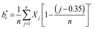
k, the three L-moment estimators of $$\hat{\lambda}_1(k), \hat{\lambda}_2(k)$$, and $$\hat{\lambda}_3(k)$$ should be computed by employing the unbiased PWM sample estimators $$b_r^*$$ [
57]:
where
n is the number of observations at site
k and $$r=0-3$$ represents the zero-, first-, second-, and third- moment. The population estimate $$\hat{\beta}_r$$ will be equal to:
The L-moments are the functions of probability weighted moments [
58]:
The parameters of the GEV distribution could be estimated in terms of L-moments [
50,
58]:
where $$\Gamma(1+\kappa)$$ is the factorial function for real and complex numbers. Having the distribution parameters computed, the GEV quantiles can be estimated as follows [
50]:
where
P is the cumulative probability of interest. For instance, a 100-year flood has a return period of 100 years with the probability of occurrence $$P=1-\frac{1}{T}=0.99$$.
The Cunnane’s plotting position [
59], is an empirical probability function suggested for visually checking the goodness-of-fit for the GEV distribution [
60]:
where
i is the rank of the observation in which
i = 1 goes with the greatest observation. The probability of occurrence is then calculated using Equation (15).
If the GEV distribution is an appropriate choice, then the plot of $$Z_{i}=\frac{X_{i}-\hat{\mu}_{X}}{\hat{\sigma}_{X}} \,\mathrm{vs.}\, \hat{X}_{P_{i}}=\xi+\frac{\alpha}{\kappa}\left\{1-\left[-\ell nP_{i}\right]^{\kappa}\right\}$$ should be close to 1:1 line [
22].
3. Results and Discussion
The results were presented in four sections for both reference and nonreference sites within HUC02 water resources regions of the contiguous US (). First, we compared and contrasted the ratio of observed peak flow to estimated flood quantiles between reference and nonreference sites. Second, we identified regions where either GEV outperformed LP3 or vice versa. Third, we analyzed how partitioning sites into reference and nonreference categories influenced the spatial distribution of shape parameters for LP3 and GEV. Finally, we reported the results of goodness-of-fit tests for both distributions, categorized by whether the site was classified as reference or nonreference.
3.1. The Ratio (R) of Observed to Estimated (Obs/Est) Flood Quantiles for Reference and Nonreference Sites
The increasing flood frequency and magnitude across the US [
61,
62], have raised concerns about selecting the appropriate flood quantile estimates [
12,
16,
63]. To investigate how disturbances affect estimated flood quantiles using LP3 or GEV, we calculated the ratio of observed peak flows to the corresponding estimated quantiles at both reference and nonreference sites for the return periods ranging from 2 to 200 years. A ratio of “Obs/Est < 1” indicates a good fit between the distribution and peak flow observations (i.e., overestimating floods). Conversely, when “Obs/Est > 1” (i.e., underestimating floods), it may raise concerns about the LP3 or GEV distributions’ capability to accurately capture floods of a specific return period ().
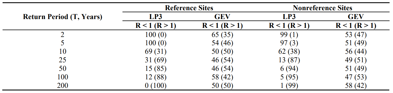
. Percentage of reference (out of 26) and nonreference (out of 78) sites for the ratio (R) of observed peak flows to the corresponding flood quantile estimates (Obs/Est). The ratio of Obs/Est < 1 represents the overestimation of flood while flood is underestimated when Obs/Est > 1.
The results showed that for reference sites, the performance of the LP3 distribution in capturing observed peak flows improved as the return period decreased. LP3 performed particularly well in estimating low flood quantiles with return periods of 2 to 25 years. Conversely, for flood quantiles with return periods of 50 to 200 years, GEV outperformed LP3 (). Both GEV and LP3 underestimated (R > 1) observed peak flows with return periods of 50 to 200 years in 42–54% and 85–100% of the reference sites, respectively (). Similar patterns were observed for nonreference sites. LP3 performed better than GEV in estimating floods with return periods of 2 to 10 years. However, for return periods of 25 to 200 years, both GEV and LP3 underestimated observed peak flows in 42–53% and 87–99% of the nonreference sites, respectively ().
3.2. Regions Where LP3 Outperformed GEV or Vice Versa
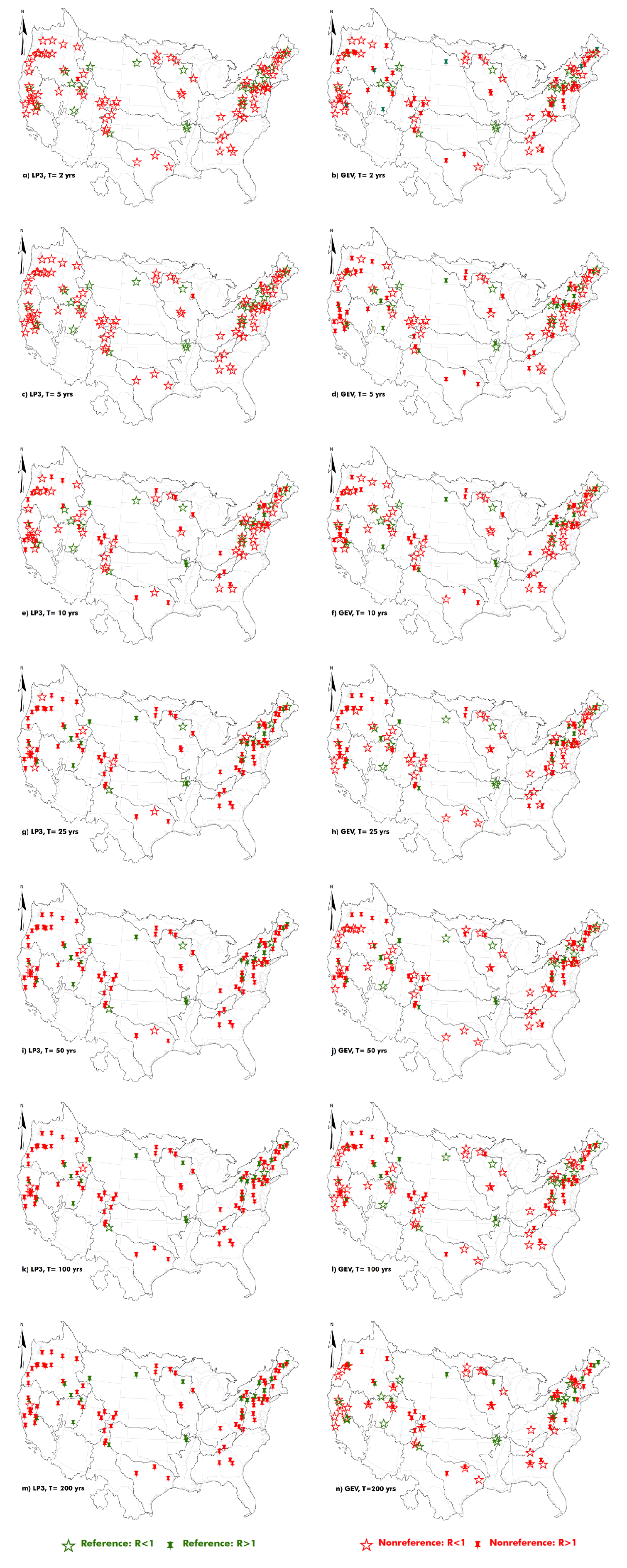
We observed no spatial pattern for floods with return periods of 2, 5, and 200 years at both reference and nonreference sites where LP3 failed to capture the observed peak flow (a,c,m). LP3 performed well for floods with a return period of 10 years at reference sites on the West coast and nonreference sites in the Northeast (e). However, LP3 estimates for return periods of 50 and 100 years matched the observed quantiles at only 10% of the study sites (i,k). Wang et al. (2011) [
39] also emphasized the superiority of the LP3 distribution over GEV in non-dam-affected sites in California. Reinders and Munoz (2024) [
21] also suggested fitting GEV to peak flows in colder and wetter climates, likely because of established high-flow regimes from year to year, while recommending the use of the log-normal distribution for dry regions, likely due to their flashy peak flow regimes.
The GEV distribution showed poor performance in estimating flood quantiles for reference sites located in the Central US (return period of 10 years, f), West US (return period of 25 years, h), South and West US (return period of 50 years, j), West US (return period of 100 years, l), and Northeast US (return period of 200 years, n). However, GEV accurately captured observed peak flow in the Northeast and Central US for floods with the return periods of 25, 50 and 100 years (h,j,l). Additionally, GEV performed well for lower flood quantiles of 2 years in the Northeast (b) and 10 years in the West US (f). Pal et al. (2022) [
64] also adopted the GEV distribution to estimate events with return periods of 2, 5, 10, 25, and 50 years over northeastern US and reported satisfactory model performance.
Figure 2. The spatial performance of LP3 and GEV distributions. R > 1 represents the underestimation of flood while flood was overestimated when R < 1.
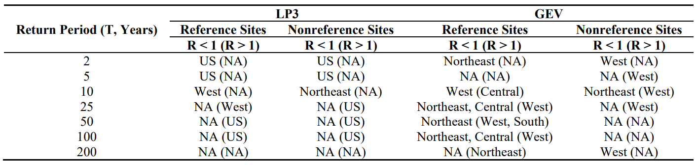
For nonreference sites, GEV effectively estimated flood quantiles with a return period of 200 years (f), but it struggled to capture peak flows with return periods of 5, 10, and 25 years in the West US (d,f,h). However, GEV performed well for smaller floods with return periods of 2 and 10 years in the West coast and Northeast, respectively (b,f). Detailed results on the regional performance of LP3 and GEV are summarized in .
. Regions that LP3 was preferred over GEV or vice versa in capturing the observed peak flow in the contiguous United States. “NA” refers to no specific region identifed.
The shape parameter (Equation (5)) plays a crucial role in accurately estimating flood quantiles with the LP3 distribution. The LP3 shape parameter is always positive as it equals the reciprocal of skewness squared. When skewness is close to zero, the shape parameter becomes a very large positive number. In Equation (8), if $$\beta<0$$, then $$\left(\frac{\beta}{\beta-1}\right)<1$$. When $$\left(\frac\beta{\beta-1}\right)$$ is raised to the power of $$\alpha $$ then $$\left(\frac{\beta}{\beta-1}\right)^\alpha<<1$$. Consequently, the LP3 estimated mean value (i.e., $$\mu_{\varrho}$$) becomes lower than the sample mean, and the distribution may fail to capture the observed peak flow accurately. Therefore, studying the variability of the shape parameter across the US will help identify regions where LP3 may not perform successfully.
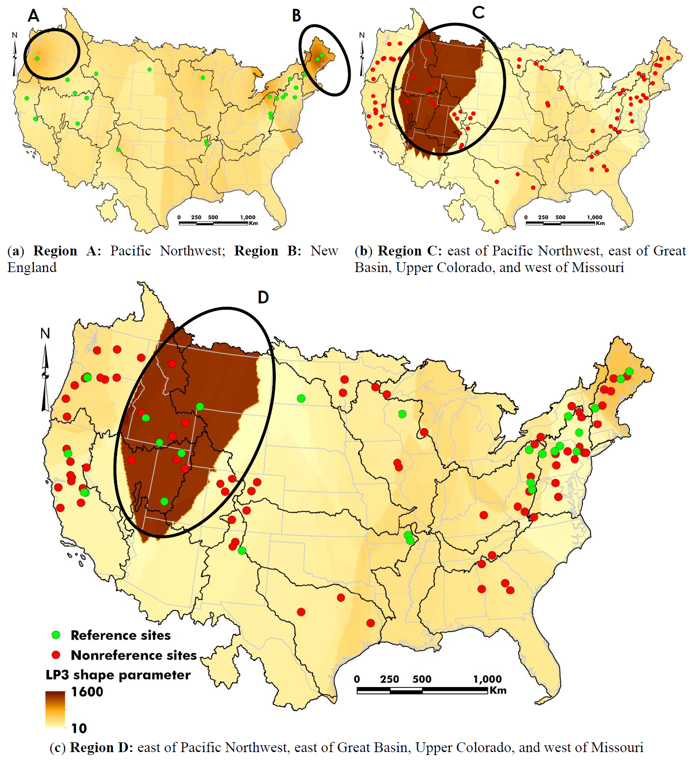
The reference sites located in the Pacific Northwest and New England regions showed the highest shape parameters for LP3 (a). For nonreference sites, the highest values of shape parameters were distributed across water resources regions east of Pacific Northwest, east of the Great Basin, Upper Colorado, and west of Missouri (b). When considering both reference and nonreference sites together, the spatial patterns of shape parameters were primarily influenced by nonreference sites (c).
Examining the shape parameters of the LP3 distribution without distinguishing between reference and nonreference sites can give a misleading impression of the effectiveness of LP3 in the Pacific Northwest and New England regions. When considering only reference sites (a), floods were underestimated in the Pacific Northwest and New England despite the high shape parameters of LP3, likely due to nonstationarity in climate. However, when both reference and nonreference sites were considered together, the LP3 shape parameter decreased in these regions, resulting in flood quantile estimates that were closer to the observed peak flows.
. The spatial pattern of shape parameter for LP3 distribution throughout the US for (<b>a</b>) reference sites, (<b>b</b>) nonreference sites, and (<b>c</b>) reference and nonreference sites together. The larger the shape parameter was, the lower the performance of LP3 distribution. The solid empty black circles identified regions with large shape parameters. The surface contours were interpolated among study sites via ordinary Krigging with spherical semivariogram model in ArcGIS.
The GEV distribution with a positive shape parameter ($$\kappa$$) has a finite upper bound. When $$\kappa>0$$ in Equation (31), the term $$\frac\alpha\kappa\left\{1-[-\ell nP]^\kappa\right\}$$ will not be large enough so that the summation with $$\xi$$ making it less likely to capture the observed peak flow. Conversely, a negative shape parameter corresponds to a distribution with a thicker right-hand tail [
50,
65]. A shape parameter of 1/3 implies that moments of order 3 and higher are infinite [
24]. When $$\kappa<0$$ in Equation (31), the term $$\frac\alpha\kappa\left\{1-[-\ell nP]^\kappa\right\}$$ becomes a large number, and the summation with $$\xi$$ will more effectively estimate the observed peak flow.
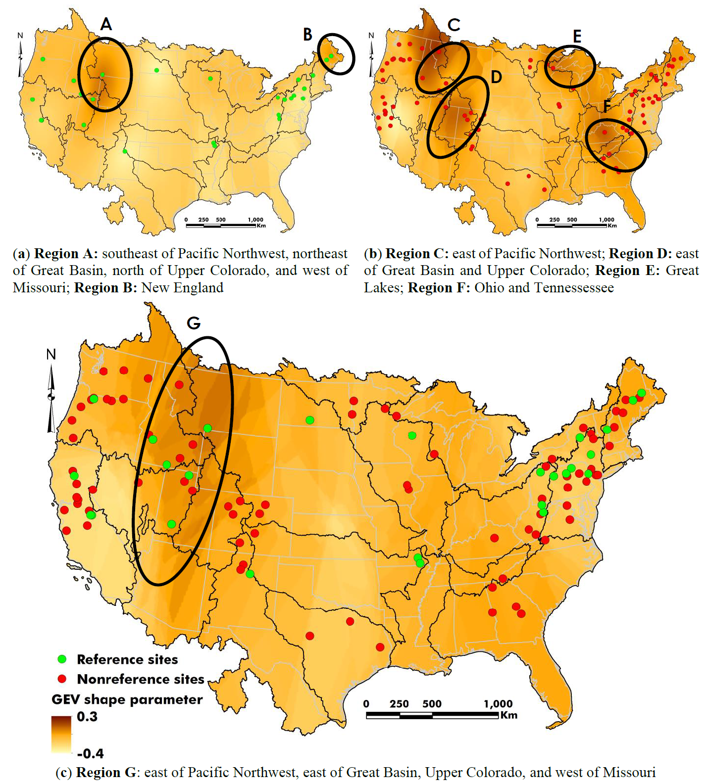
At reference sites, the GEV shape parameter was predominantly positive in the southeast of the Pacific Northwest, northeast of the Great Basin, north of Upper Colorado, west of Missouri, and New England regions (a). As mentioned earlier, a positive shape parameter ($$\kappa>0$$) in GEV distributions increases the likelihood of underestimating floods. For nonreference sites, positive shape parameters were observed in the east of the Pacific Northwest, east of the Great Basin, Upper Colorado, Great Lakes, Ohio, and Tennessee water resources regions (b). However, without distinguishing between reference and nonreference sites, the spatial pattern of the GEV shape parameter did not precisely align with either category (c).
. The spatial pattern of shape parameter for GEV distribution throughout the US for (<b>a</b>) reference sites, (<b>b</b>) nonreference sites, and (<b>c</b>) reference and nonreference sites together. In regions with negative shape parameter, GEV performed better in capturing the observed peak flow. The solid empty black circles identified regions with large shape parameters. The surface contours were interpolated among study sites via ordinary Krigging with spherical semivariogram model in ArcGIS.
Similar to the LP3 results, combining reference and nonreference sites can lead to misleading conclusions. Regions C and D (b) exhibited higher positive shape parameters compared to Region A (a), suggesting a greater likelihood of underestimating flood quantiles in those regions. Region G (c), which encompassed Regions A, C, and D showed shape parameters with magnitudes similar to Region A, indicating that GEV might estimate floods closer to observed peak flows in Region G. However, when compared to Region C and D (b) with higher positive shape parameters and a higher chance of underestimating floods, it becomes clear that the combining results from reference and nonreference sites can potentially lead to misleading interpretations.
3.4. Goodness-of-Fit
The goodness-of-fit test evaluates how well a distribution fits the peak flow observations and provides insights into the explanatory power of the distribution [
49]. It does not, however, ascertain the true population distribution. Empirical probabilities for LP3 and GEV distributions were estimated using the Blom’s and Cunnane’s empirical probability functions (Equations (14) and (32)). Following the approach suggested by Serago and Vogel (2018) [
22], we conducted a goodness-of-fit test. The cross-correlation coefficients between observed and estimated flood quantiles, summarized in , ranged from 0.8157–0.9986, indicating high correlations for both reference and nonreference sites. It suggests that LP3 and GEV distributions can effectively estimate flood quantiles across the US.
Table 3. The cross-correlation range of the goodness-of-fit test for the LP3 and GEV distributions.
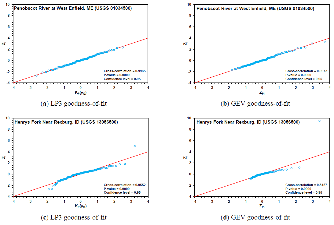
It is important to interpret the goodness-of-fit results with caution, as the test only assesses whether LP3 or GEV distributions adequately fit the observed data and not necessarily the true population distribution. As discussed earlier, there were regions across the US where LP3 and GEV did not perform well in estimating flood quantiles. Particularly, critical flows, such as those with larger return periods, may not be accurately estimated by these distributions. This can potentially lead to incidents and failures during the operational life of hydraulic structures, such as large dams. Examples of the goodness-of-fit tests for LP3 and GEV distributions are presented in . These illustrations help visualize how well these distributions match the observed peak flow data.
. Examples of goodness-of-fit for LP3 and GEV distributions tested at reference (<b>a</b>,<b>b</b>) and nonreference (<b>c</b>,<b>d</b>) sites. Despite the closeness of cross-correlation values to “1”, LP3 or GEV might not be able to capture high or low flows (<b>c</b>,<b>d</b>).
4. Summary and Conclusions
This study aimed to understand how spatial heterogeneity influences the choice of statistical distribution for flood frequency analysis in undisturbed and disturbed watersheds across the US. We used LP3 and GEV distributions to estimate flood quantiles at 26 reference and 78 nonreference sites throughout the contiguous US, each with more than 100 years of record. Comparing results from reference and nonreference sites provided insights into the effects of climate and anthropogenic factors such as land use/cover change, river regulation, irrigation, water withdrawal, and urbanization on flood frequency analysis.
We compared observed peak flows to estimated quantiles for return periods ranging from 2 to 200 years. For design purposes, LP3 distribution provided more reliable flood quantile estimates for return periods of 2 to 10 years, whereas caution is advised when using LP3 estimates for return periods exceeding 50 years. Conversely, GEV performed better than LP3 in estimating floods with return periods of 50 years or more. The reliability of GEV estimates for return periods of 10 years or less varied regionally and might be more effectively substituted with LP3 estimates. Spatial variations in LP3 or GEV performance corroborates the findings of Reinders and Munoz (2024) [
21], indicating the importance of considering hydroclimatic properties when selecting an appropriate distribution for flood frequency analysis, rather than solely relying on LP3 as a nationally suggested distribution.
The shape parameter of the LP3 distribution exhibited spatial variability depending on whether the study site was a reference or nonreference site. In regions such as the Pacific Northwest, Great Basin, Upper Colorado, Missouri, and New England, the LP3 flood quantile estimates may not be reliable due to higher values of the shape parameters compared to other regions in the US. Conversely, in regions where LP3 flood quantile estimates were not reliable, the GEV distribution with a negative shape parameter effectively captured observed floods. Our findings emphasize the importance of distinguishing between reference and nonreference sites when reporting the shape parameters of both LP3 and GEV distributions. Accurate estimates of flood quantiles are crucial for safeguarding infrastructure throughout its service life, thereby minimizing potential loss of life, property damage, and infrastructure failures.
The goodness-of-fit tests determined whether LP3 or GEV could represent the true population distribution. However, caution is needed when interpreting high cross-correlation values from these tests, as the performance of LP3 and GEV distributions may differ significantly depending on whether the site is a reference or nonreference site.
Future studies can integrate stations with less than 100 years of record and explore record extension procedures such as MOVE [
15,
66]. Instead of relying solely on GEV and LP3 distributions, frequency analysis can utilize alternative statistical distributions (e.g., those available in RMC BestFit v1.0 developed by USACE, available at: https://www.rmc.usace.army.mil/Software/RMC-BestFit/). Considering partial duration series to augment data points for upper tercile flows could also be explored at stream gauge stations with less than 30 years of information (e.g., Berton and Rahmani (2024) [
67]).
Supplementary Materials
The following supporting information can be found at: https://www.sciepublish.com/article/pii/251, Table S1: The description of 26 reference and 78 nonreference study sites with more than 100 years of peak flow data across the contiguous United States.
Acknowledgments
Authors would like to acknowledge and extent their gratitude for the support provided by Kansas State University for the current research. The work was conducted between 2018–2019, during Dr. Berton’s tenure as a postdoctoral fellow and Dr. Rahmani’s tenure as an assistant professor in the Department of Biological and Agricultural Engineering at Kansas State University.
Author Contributions
R.B.: Conceptualization, Methodology, Software, Validation, Formal Analysis, Investigation, Data Curation, Writing—Original Draft Preparation, Writing–Review & Editing, Visualization; V.R.: Conceptualization, Validation, Resources, Writing—Review & Editing, Supervision, Project Administration, Funding Acquisition.
Ethics Statement
Not applicable.
Informed Consent Statement
Not applicable.
Funding
This research was funded by the Department of Biological and Agricultural Engineering at Kansas State University through the contribution number of “19-102-J” of the Kansas Agricultural Experiment Station.
Declaration of Competing Interest
The authors declare that they have no known competing financial interests or personal relationships that could have appeared to influence the work reported in this paper. Addtionally, the views expressed in this paper are those of the authors and do not necessarily reflect the official positions or opinions of their affiliated institutions.
References
1.
Hallegatte S, Green C, Nicholls RJ, Corfee-Morlot J. Future flood losses in major coastal cities.
Nat. Clim. Chang. 2013,
3, 802–806. doi:10.1038/nclimate1979.
[Google Scholar]
2.
Saharia M, Kirstetter P-E, Vergara H, Gourley JJ, Hong Y. Characterization of floods in the United States.
J. Hydrol. 2017,
548, 524–535. doi:10.1016/j.jhydrol.2017.03.010.
[Google Scholar]
3.
Sanders BF, Schubert JE, Kahl DT, Mach KJ, Brady D, AghaKouchak A, et al. Large and inequitable flood risks in Los Angeles, California.
Nat. Sustain. 2022,
6, 47–57. doi:10.1038/s41893-022-00977-7.
[Google Scholar]
4.
Qiang Y, Lam NS.N, Cai H, Zou L. Changes in Exposure to Flood Hazards in the United States.
Ann. Am. Assoc. Geogr. 2017,
107, 1332–1350. doi:10.1080/24694452.2017.1320214.
[Google Scholar]
5.
Pielke RA, Downton MW. Precipitation and Damaging Floods: Trends in the United States, 1932–1997.
J. Clim. 2000,
13, 3625–3637. doi:10.1175/1520-0442(2000)013<3625:PADFTI>2.0.CO;2.
[Google Scholar]
6.
Berton R, Driscoll CT, Chandler DG. Changing climate increases discharge and attenuates its seasonal distribution in the northeastern United States.
J. Hydrol. Reg. Stud. 2016,
5, 164–178. doi:10.1016/j.ejrh.2015.12.057.
[Google Scholar]
7.
Hoerling M, Eischeid J, Perlwitz J, Quan X-W, Wolter K, Cheng L. Characterizing Recent Trends in U.S. Heavy Precipitation.
J. Clim. 2016,
29, 2313–2332. doi:10.1175/JCLI-D-15-0441.1.
[Google Scholar]
8.
Ivancic TJ, Shaw SB. Examining why trends in very heavy precipitation should not be mistaken for trends in very high river discharge.
Clim. Chang. 2015,
133, 681–693. doi:10.1007/s10584-015-1476-1.
[Google Scholar]
9.
Rahmani V, Hutchinson SL, Harrington JA, Hutchinson JMS. Analysis of frequency and magnitude of extreme rainfall events with potential impacts on flooding: A case study from the central United States: Extreme rainfall events with potential impacts on flooding.
Int. J. Climatol. 2016,
36, 3578–3587. doi:10.1002/joc.4577.
[Google Scholar]
10.
Kim H, Villarini G. Higher emissions scenarios lead to more extreme flooding in the United States.
Nat. Commun. 2024,
15, 237. doi:10.1038/s41467-023-44415-4.
[Google Scholar]
11.
Knotters M, Bokhove O, Lamb R, Poortvliet PM. How to cope with uncertainty monsters in flood risk management?
Camb. Prisms Water 2024,
2, e6. doi:10.1017/wat.2024.4.
[Google Scholar]
12.
Maurer EP, Kayser G, Doyle L, Wood AW. Adjusting Flood Peak Frequency Changes to Account for Climate Change Impacts in the Western United States.
J. Water Resour. Plan. Manag. 2018,
144, 05017025. doi:10.1061/(ASCE)WR.1943-5452.0000903.
[Google Scholar]
13.
Pirone D, Cimorelli L, Pianese D. The effect of flood-mitigation reservoir configuration on peak-discharge reduction during preliminary design.
J. Hydrol. Reg. Stud. 2024,
52, 101676. doi:10.1016/j.ejrh.2024.101676.
[Google Scholar]
14.
Sanchez GM, Petrasova A, Skrip MM, Collins EL, Lawrimore MA, Vogler JB, et al. Spatially interactive modeling of land change identifies location-specific adaptations most likely to lower future flood risk.
Sci. Rep. 2023,
13, 18869. doi:10.1038/s41598-023-46195-9.
[Google Scholar]
15.
England JF, Jr., Cohn TA, Faber BA, Stedinger JR, Thomas WO, Jr., Veilleux AG; et al. Guidelines for Determining Flood Flow Frequency—Bulletin 17C (Report No. 4-B5), Techniques and Methods; US Geological Survey: Reston, VA, USA, 2019; doi:10.3133/tm4B5.
16.
Hodgkins GA, Dudley RW, Archfield SA, Renard B. Effects of climate, regulation, and urbanization on historical flood trends in the United States.
J. Hydrol. 2019,
573, 697–709. doi:10.1016/j.jhydrol.2019.03.102.
[Google Scholar]
17.
Falcone JA, Carlisle DM, Wolock DM, Meador MR. GAGES: A stream gage database for evaluating natural and altered flow conditions in the conterminous United States.
Ecology 2010,
91, 621. doi:10.1890/09-0889.1.
[Google Scholar]
18.
Boscarello L, Ravazzani G, Cislaghi A, Mancini M. Regionalization of Flow-Duration Curves through Catchment Classification with Streamflow Signatures and Physiographic–Climate Indices.
J. Hydrol. Eng. 2015,
21, 05015027. doi:10.1061/(ASCE)HE.1943-5584.0001307.
[Google Scholar]
19.
Chiverton A, Hannaford J, Holman I, Corstanje R, Prudhomme C, Bloomfield J, et al. Which catchment characteristics control the temporal dependence structure of daily river flows?
Hydrol. Process. 2015,
29, 1353–1369. doi:10.1002/hyp.10252.
[Google Scholar]
20.
Jean Louis M, Crosato A, Mosselman E, Maskey S. Effects of urbanization and deforestation on flooding: Case study of Cap-Haïtien City, Haiti. J. Flood Risk Manag. 2024, e13020. doi:10.1111/jfr3.13020.
21.
Reinders JB, Munoz SE. Accounting for hydroclimatic properties in flood frequency analysis procedures.
Hydrol. Earth Syst. Sci. 2024,
28, 217–227. doi:10.5194/hess-28-217-2024.
[Google Scholar]
22.
Serago JM, Vogel RM. Parsimonious nonstationary flood frequency analysis.
Adv. Water Resour. 2018,
112, 1–16. doi:10.1016/j.advwatres.2017.11.026.
[Google Scholar]
23.
Serinaldi F, Kilsby CG. Stationarity is undead: Uncertainty dominates the distribution of extremes.
Adv. Water Resour. 2015,
77, 17–36. doi:10.1016/j.advwatres.2014.12.013.
[Google Scholar]
24.
Villarini G, Smith JA. Flood peak distributions for the eastern United States.
Water Resour. Res. 2010,
46, W06504. doi:10.1029/2009WR008395.
[Google Scholar]
25.
Barth NA, Villarini G, Nayak MA, White K. Mixed populations and annual flood frequency estimates in the western United States: The role of atmospheric rivers.
Water Resour. Res. 2017,
53, 257–269. doi:10.1002/2016WR019064.
[Google Scholar]
26.
Griffis VW, Stedinger JR. Log-Pearson Type 3 Distribution and Its Application in Flood Frequency Analysis. I: Distribution Characteristics.
J. Hydrol. Eng. 2007,
12, 482–491. doi:10.1061/(ASCE)1084-0699(2007)12:5(482).
[Google Scholar]
27.
Hosking JRM, Wallis JR, Wood EF. Estimation of the Generalized Extreme-Value Distribution by the Method of Probability-Weighted Moments.
Technometrics 1985,
27, 251–261. doi:10.1080/00401706.1985.10488049.
[Google Scholar]
28.
Hu L, Nikolopoulos EI, Marra F, Anagnostou EN. Sensitivity of flood frequency analysis to data record, statistical model, and parameter estimation methods: An evaluation over the contiguous United States.
J. Flood Risk Manag. 2020,
13, e12580. doi:10.1111/jfr3.12580.
[Google Scholar]
29.
Karim MA, Chowdhury JU. A comparison of four distributions used in flood frequency analysis in Bangladesh.
Hydrol. Sci. J. 1995,
40, 55–66. doi:10.1080/02626669509491390.
[Google Scholar]
30.
Lamontagne JR, Stedinger JR. Examination of the Spencer-McCuen Outlier-Detection Test for Log-Pearson Type 3 Distributed Data.
J. Hydrol. Eng. 2016,
21, 04015069. doi:10.1061/(ASCE)HE.1943-5584.0001321.
[Google Scholar]
31.
Miniussi A, Marani M, Villarini G. Metastatistical Extreme Value Distribution applied to floods across the continental United States.
Adv. Water Resour. 2020,
136, 103498. doi:10.1016/j.advwatres.2019.103498.
[Google Scholar]
32.
Pal S, Wang J, Feinstein J, Yan E, Kotamarthi VR. Projected changes in extreme streamflow and inland flooding in the mid-21st century over Northeastern United States using ensemble WRF-Hydro simulations.
J. Hydrol. Reg. Stud. 2023,
47, 101371. doi:10.1016/j.ejrh.2023.101371.
[Google Scholar]
33.
Persiano S, Salinas JL, Stedinger JR, Farmer WH, Lun D, Viglione A, et al. A comparison between generalized least squares regression and top-kriging for homogeneous cross-correlated flood regions.
Hydrol. Sci. J. 2021,
66, 565–579. doi:10.1080/02626667.2021.1879389.
[Google Scholar]
34.
Roy B, Islam AKMS, Islam GMT, Khan, MdJU, Bhattacharya B, Ali MdH, et al. Frequency Analysis of Flash Floods for Establishing New Danger Levels for the Rivers in the Northeast
Haor Region of Bangladesh.
J. Hydrol. Eng. 2019,
24, 05019004. doi:10.1061/(ASCE)HE.1943-5584.0001760.
[Google Scholar]
35.
Saf B. Regional Flood Frequency Analysis Using L-Moments for the West Mediterranean Region of Turkey.
Water Resour. Manag. 2009,
23, 531–551. doi:10.1007/s11269-008-9287-z.
[Google Scholar]
36.
Sampaio J, Costa V. Bayesian regional flood frequency analysis with GEV hierarchical models under spatial dependency structures.
Hydrol. Sci. J. 2021,
66, 422–433. doi:10.1080/02626667.2021.1873997.
[Google Scholar]
37.
Vidrio-Sahagún CT, Ruschkowski J, He J, Pietroniro A. A practice-oriented framework for stationary and nonstationary flood frequency analysis.
Environ. Model. Softw. 2024,
173, 105940. doi:10.1016/j.envsoft.2024.105940.
[Google Scholar]
38.
Walshaw D. Generalized Extreme Value Distribution. In Wiley StatsRef: Statistics Reference Online; Balakrishnan N, Colton T, Everitt B, Piegorsch W, Ruggeri F, Teugels JL, Eds.; Wiley Online Library: Hoboken, NJ, USA, 2014; p. 11.
39.
Wang W, Wang X-G, Zhou X. Impacts of Californian dams on flow regime and maximum/minimum flow probability distribution.
Hydrol. Res. 2011,
42, 275–289. doi:10.2166/nh.2011.137.
[Google Scholar]
40.
Yu X, Cohn TA, Stedinger JR. Flood Frequency Analysis in the Context of Climate Change. In World Environmental and Water Resources Congress 2015. Presented at the World Environmental and Water Resources Congress 2015; American Society of Civil Engineers: Austin, TX, USA, 2015; pp. 2376–2385. doi:10.1061/9780784479162.233.
41.
Falcone J. GAGES-II: Geospatial Attributes of Gages for Evaluating Streamflow (Vector Digital Data); U.S. Geological Survey: Reston, VA, USA, 2011. doi:10.3133/70046617.
42.
Lins HF. USGS Hydro-Climatic Data Network 2009 (HCDN–2009) (Fact Sheet); U. S. Geological Survey: Reston, VA, USA, 2012.
43.
U.S. Water Resources Council. Water Resources Regions and Subregions for the National Assessment of Water and Related Land Resources; Water Resources Council: Washington, DC, USA, 1970.
44.
Micevski T, Hackelbusch A, Haddad K, Kuczera G, Rahman A. Regionalisation of the parameters of the log-Pearson 3 distribution: A case study for New South Wales, Australia.
Hydrol. Process. 2015,
29, 250–260. doi:10.1002/hyp.10147.
[Google Scholar]
45.
Vogel RM, Fennessey NM. L moment diagrams should replace product moment diagrams.
Water Resour. Res. 1993,
29, 1745–1752. doi:10.1029/93WR00341.
[Google Scholar]
46.
Izinyon O, Ehiorobo J. L-moments approach for flood frequency analysis of river Okhuwan in Benin-Owena River basin in Nigeria.
Niger. J. Technol. 2014,
33, 10. doi:10.4314/njt.v33i1.2.
[Google Scholar]
47.
Rootzén H, Katz RW. Design Life Level: Quantifying risk in a changing climate: Design Life Level.
Water Resour. Res. 2013,
49, 5964–5972. doi:10.1002/wrcr.20425.
[Google Scholar]
48.
Stedinger JR. Flood frequency analysis. In Handbook of Applied Hydrology; Singh VP, Ed.; McGraw Hill Book Co.: Ann Arbor, MI, USA, 2016.
49.
Vogel RM, Wilson I. Probability distribution of annual maximum, mean, and minimum streamflows in the united states.
J. Hydrol. Eng. 1996,
1, 69–76. doi:10.1061/(ASCE)1084-0699(1996)1:2(69).
[Google Scholar]
50.
Stedinger JR, Vogel RM, Foufoula-Georgiou E. Frequency analysis of extreme events. In Handbook of Hydrology; Maidment DR, Ed.; McGraw-Hill, the University of Michigan: Ann Arbor, MI, USA, 1993; p. 1424.
51.
Bobée B. The Log Pearson type 3 distribution and its application in hydrology.
Water Resour. Res. 1975,
11, 681–689. doi:10.1029/WR011i005p00681.
[Google Scholar]
52.
Derenzo SE. Approximations for Hand Calculators Using Small Integer Coefficients.
Math. Comput. 1977,
31, 214–222. doi:10.2307/2005791.
[Google Scholar]
53.
Vogel RM, Kroll CN. Low-Flow Frequency Analysis Using Probability-Plot Correlation Coefficients.
J. Water Resour. Plan. Manag. 1989,
115, 338–357. doi:10.1061/(ASCE)0733-9496(1989)115:3(338).
[Google Scholar]
54.
Jenkinson AF. The frequency distribution of the annual maximum (or minimum) values of meteorological elements.
Q. J. R. Meteorol. Soc. 1955,
81, 158–171. doi:10.1002/qj.49708134804.
[Google Scholar]
55.
Wallis JR. Risk and uncertainties in the evaluation of flood events for the design of hydraulic structures. In Piene e Siccita, Fondazione Politec; Guggino GR, Todini E, Eds.; Del Mediterr: Catania, Italy, 1980; pp. 3–36.
56.
Greis NP, Wood EF. Regional flood frequency estimation and network design.
Water Resour. Res. 1981,
17, 1167–1177. doi:10.1029/WR017i004p01167.
[Google Scholar]
57.
Greenwood JA, Landwehr JM, Matalas NC, Wallis JR. Probability weighted moments: Definition and relation to parameters of several distributions expressable in inverse form.
Water Resour. Res. 1979,
15, 1049–1054. doi:10.1029/WR015i005p01049.
[Google Scholar]
58.
Hosking JRM. L-Moments: Analysis and Estimation of Distributions Using Linear Combinations of Order Statistics.
J. R. Stat. Soc. Ser. B Methodol. 1990,
52, 105–124. doi: 10.1111/j.2517-6161.1990.tb01775.x.
[Google Scholar]
59.
Cunnane C. Unbiased plotting positions—A review.
J. Hydrol. 1978,
37, 205–222. doi:10.1016/0022-1694(78)90017-3.
[Google Scholar]
60.
Chowdhury JU, Stedinger JR. Confidence Interval for Design Floods with Estimated Skew Coefficient.
J. Hydraul. Eng. 1991,
117, 811–831. doi:10.1061/(ASCE)0733-9429(1991)117:7(811).
[Google Scholar]
61.
Berghuijs WR, Aalbers EE, Larsen JR, Trancoso R, Woods RA. Recent changes in extreme floods across multiple continents.
Environ. Res. Lett. 2017,
12, 114035. doi:10.1088/1748-9326/aa8847.
[Google Scholar]
62.
Slater LJ, Villarini G. Recent trends in U.S. flood risk.
Geophys. Res. Lett. 2016,
43, 12428–12436. doi:10.1002/2016GL071199.
[Google Scholar]
63.
Salas J, Obeysekera J. Revisiting the Concepts of Return Period and Risk for Nonstationary Hydrologic Extreme Events.
J. Hydrol. Eng. 2014,
19, 554–568.
[Google Scholar]
64.
Pal S, Wang J, Feinstein J, Yan E, Kotamarthi VR. Projected Increase in Hydrologic Extremes in the Mid-21st Century for Northeastern United States (preprint). Hydrology 2022, doi:10.1002/essoar.10511327.1.
65.
Hosking JRM, Wallis JR. Regional Frequency Analysis: An Approach Based on L-Moments; Cambridge University Press: Cambridge, UK, 2005.
66.
Hirsch RM. A comparison of four streamflow record extension techniques.
Water Resour. Res 1982,
18, 1081–1088. doi:10.1029/WR018i004p01081.
[Google Scholar]
67.
Berton R, Rahmani V. Improving Low-Frequency Flood Estimation Using the Partial Duration Series Instead of the Annual Maximum Across the United States.
Adv. Hydrol. Meteorol. 2024,
1, 14. doi:10.33552/AHM.2024.01.000523.
[Google Scholar]
 Vahid Rahmani
2
Vahid Rahmani
2