1. Introduction
Several indicators have shown that there is poor water resource management in terms of its availability and distribution in West African countries [
1]. Despite its paramount importance and crucial role in supporting livelihoods, agriculture, and ecosystems. This condition is expected to worsen with increasing pressures from population growth, urbanization, and climate change [
2]. Though effective management of the water resources, including accurate streamflow forecasting, is essential for sustainable water resource development and resilience under various stressors in the region [
3]. The prediction of water flow in rivers and streams under the currently identified stressors is critical for informed decisions related to various sectors of the economy, such as agriculture [
4,
5], water supply [
6,
7], hydropower generation [
8], and disaster risk reduction [
9]. In terms of agriculture, accurate streamflow forecasts are critical for planning irrigation schedules, managing water resources, and mitigating the impacts of droughts and floods on crops. A lot of farmers depend on timely and reliable information to make informed decisions about planting periods, irrigation water demand, and harvesting patterns [
10]. If this is achieved, it will improve agricultural productivity while minimizing risks. Furthermore, many water resource management authorities in the region require streamflow forecasts to allocate water resources efficiently by balancing competing water demands and guaranteeing sustainable water supply for domestic, industrial, and environmental purposes [
11]. Another significant sector in which the application of streamflow forecasting is seriously required is hydropower generation, as many countries in the region rely on it as a primary source of electricity. It enables hydropower operators to optimise reservoir operations, manage water releases, and plan the quantity of electricity generation [
12]. Thereby maximising energy production and minimising disruptions, as noticed in many countries in the region. Accurate forecasts are essential for balancing energy supply and demand, particularly during periods of peak consumption or low water availability [
13].
In addition to supporting socio-economic activities, streamflow forecasting plays an important role in disaster risk reduction and climate resilience efforts in West Africa [
10]. Appropriate and accurate forecasts can help decision-makers anticipate and respond to hydrological related hazards, such as floods and droughts [
14]. It further guides the implementation of early warning systems, prevention of disaster by evacuating at-risk communities, and implementing measures to protect infrastructure and livelihoods [
15]. Additionally, integrating streamflow forecasts into disaster risk management strategies in West African countries can enhance their resilience to climate-related hazards and reduce the socio-economic impacts of extreme events [
16].
Over the past few years, progress in optimization techniques has contributed to substantial advances in streamflow forecasting accuracy and reliability [
17]. These techniques include machine learning models and hybrid optimisation algorithms, which have shown the potential of hydrological prediction. Although several optimisation algorithms are evolving, and many are yet to be utilised for streamflow prediction. According to Rajwar, et al. [
18], there are more than 500 nature-inspired optimisation algorithms known as meta-heuristic algorithms (MA) in existence, but only a few are utilised for streamflow prediction [
19]. For example, machine learning models such as adaptive neuro-fuzzy inference system (ANFIS), artificial neural networks (ANNs), multilayer perceptron (MLP), random forest (RF), support vector regression (SVR), and long short-term memory (LSTM) networks have shown promise in capturing complex relationships and patterns in streamflow data [
20,
21,
22]. However, the performance of machine learning models relies on the optimisation of model parameters and hyperparameters, which can be challenging due to the high-dimensional and nonlinear nature of the optimisation problem [
23].
On the other hand, hybrid optimisation algorithms, which combine elements of different optimisation techniques, offer a powerful approach to streamflow forecasting optimization. These algorithms integrate machine learning models with metaheuristic optimisation algorithms, such as grey wolf optimisation (GWO), particle swarm optimisation (PSO), genetic algorithm (GA), simulated annealing (SA), differential evolution (DE), particle swarm optimisation (PSO), and other MA’s, to achieve superior performance and robustness [
24]. By leveraging hybrid algorithms’ strengths, individual methods’ limitations can be overcome, while accurate and reliable streamflow forecasts can be produced. Currently, there has been growing interest in optimisation algorithms inspired by natural phenomena, such as those based on MA’s principles, to enhance streamflow forecasting. These optimization algorithms mimic the behavior of natural processes to efficiently solve complex optimization problems, offering the potential to improve the accuracy and reliability of streamflow predictions. Additionally, advancements in related optimisation techniques, such as the Chaotic Grey Wolf Optimisation (CGWO) algorithm, immune-inspired algorithms, the Adaptive Fast Orthogonal Search (FOS) algorithm, the Butterfly optimisation algorithm, and many more, have provided further opportunities for streamflow forecasting [
25]. But a recent study shows that PSO often suffers from premature convergence due to velocity-position updates, leading to stagnation in local optima [
26]. GA, while effective, relies on computationally expensive selection, crossover, and mutation processes, requiring extensive tuning [
27]. The GWO is constrained by its hierarchical structure, limiting its search diversity in complex, nonlinear problems [
28].
Since many meta-heuristic algorithms (MA) are yet to be tested for streamflow prediction, this study employs four MA hybrids in support vector machine (SVM) to predict streamflow. Meanwhile, the ultimate goal of applying hybrid optimisation techniques to streamflow predictions is to efficiently utilise well-trained MA algorithms to forecast streamflow in real-world scenarios, enhancing the efficiency of hydrologists and water resource engineers. The selection of four MA’s (the BSMA, AVOA, AA, and IIFA) over PSO, GA, and GWO is based on their superior exploration-exploitation balance, adaptability, and computational efficiency in optimizing SVR for streamflow prediction. Their adaptive parameter control mechanisms enhance predictive accuracy while reducing computational overhead, making them ideal for streamflow forecasting [
29].
However, conventional MAs often lack explicit equations that can be directly utilised by experts. As a substitute, researchers naturally need to check the algorithms that can be restructured or modified to meet desired needs, which can be difficult due to the requirement for programming skills. Not only that, the computational time and parameter adjustments for optimal output and precision in most machine learning models make them weak at providing the desired results [
30]. To address this challenge, coupling ML and MAs to overcome the intricateness of the ML model and, at the same time, opening the capabilities of several MA’s will continue to open ways for reliable prediction in water sciences [
31]. Therefore, in West Africa, where hydrological variability is high, and data availability is often limited, these approaches may offer valuable insight for enhancing streamflow prediction capabilities in the region.
However, there has not been a report on the application of many MA in the prediction of streamflows and the assessment of their capabilities in dealing with hydrological issues. Furthermore, while several studies have applied metaheuristic algorithms to machine learning models in hydrology, a direct comparison of multiple novel algorithms for SVR-based streamflow prediction remains limited. This research contributes to the field by systematically evaluating the performance of different optimization techniques and identifying the most suitable approach for enhancing SVR predictions. The results provide valuable insights into the potential of hybridizing machine learning with metaheuristics for improving hydrological forecasting models. To this end, this study is the first to integrate four novel meta-heuristic algorithms—Archery Algorithm (AA), African Vulture Optimisation Algorithm (AVOA), Binary Slime Mould Algorithm (BSMA), and Intelligent Ice Fishing Algorithm (IIFA)—into the Support Vector Machine (SVM) framework for streamflow prediction in West Africa. This study provides a comprehensive evaluation of these hybrid models, using multiple statistical metrics to assess their predictive accuracy, and compares their performance against conventional SVM models.
The study utilises some input combinations of scenarios using the time lag method, including daily streamflows, rainfall, and minimum and maximum temperature. For clear comprehension, these approaches cover the simple SVM and hybrid integrative (SVM-AA, SVM-AVOA, SVM-BSMA, and SVM-IIFA) models. In each case, the results obtained from the models are compared to check their effect and influence on enhancing the accuracy of the results. This research seeks to contribute to the advancement of streamflow forecasting techniques and provide valuable insights into the optimization of machine learning models for hydrological prediction. The findings of this study are expected to provide insight into decision-making processes in water resource management for agriculture, energy production, and disaster risk reduction purposes in the region.
2. Material and Methods
2.1. Machine Learning (ML) and Meta-Heuristic Models (MA)
This section describes the methodology for developing hybrid forecast models and introduces the performance evaluation criteria. The study considered two types of forecast models: SVM (Support Vector Machine), enhanced with a meta-heuristic algorithm (), including AA (Archery Algorithms), AVOA (African Vulture Optimization Algorithm), BSMA (Binary Slime Mould Algorithm), and IIFA (Intelligent Ice Fishing Algorithms). The hybrid models were developed exclusively for simulation purposes, aimed at predicting streamflow under historical time steps. For this purpose, SVM hybrid-based models similar to Bahramifar, et al. [
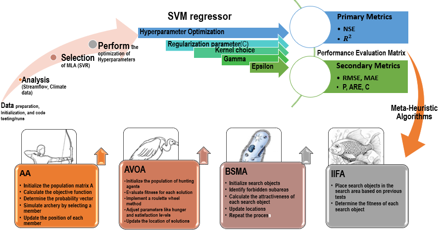
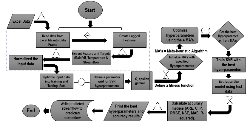
32] were adopted. Due to the increase in data mining and the capability to utilize large amounts of data for scientific inferences, ML methods have become useful tools for analyzing data for future reference. Combining ML and MA algorithms is helpful when you have a lot of complex scenarios representing the natural sequences of the climate data, and it’s hard to figure out the relationships. These methods are mostly based on data-driven processes and involve using data science to understand possible future occurrences. How well combining an ML method and MA works depends on the quality of the training data and how well it can find the relationships and information underneath. ML algorithms are different from traditional models because they don’t use predetermined mathematical equations to find patterns in data. Instead, they use computer techniques and sequences. The MA is often used when the search space for hyperparameters in machine learning (ML) algorithms is large, complex and traditional optimization methods are inadequate. In this study, two MLs (SVM) are selected () and combined with four meta-heuristic algorithms that are used to optimize the hyperparameters of SVM to enhance the performance and prediction of the streamflow.
. Simplify concept of the Methodology used in this study.
. A flowchart of the Hybrid Models integration process.
2.1.1. Support Vector Machine (SVM)
SVM’s purpose is to find the optimum hyperplane that splits classes in feature space [
33]. It is considered the most rigorous parameter-tuning ML model and tends to have a larger number of hyperparameters that require more careful tuning to achieve optimal performance. To tune these parameters like kernel choice and the regularization parameter (C) are critical for realizing the right equilibrium between model complexity and generalization. Although the SVMs can handle high-dimensional data efficiently, but the choice of kernel and other hyperparameters becomes more critical as the dimensionality increases [
34]. In a linear SVM, the aim is to find the optimal hyperplane that separates the data into different classes. This hyperplane is defined as;
where
w is the weight vector perpendicular to the hyperplane and
b is the bias term. In this case, the weight vector
w determines the orientation of the hyperplane in the feature space. When an input data
x is given, its class label is determined by which side of the hyperplane it falls on after computing $$w^{T} x + b$$. The SVM algorithm learns the optimal values for
w during the training process.
For classification, an input
x is assigned a class based on which side of the hyperplane it falls on. The optimal values of
w and
b are learned during the training process by solving an optimization problem.
For non-linearly separable data, SVM employs a kernel function $$K \left( x , x^{\prime} \right)$$ to transform the input features into a higher-dimensional space, where a linear separation can be achieved. The decision function, in this case, is defined as:
where
αi is term as the Lagrange multipliers derived by solving the dual optimization problem.
Both classification (Support Vector Classification, SVC) and regression (Support Vector Regression, SVR) applications can use the versatile Support Vector Machine (SVM) [
35]. The selection of the kernel and other hyperparameters plays an integral part in attaining the best possible performance, particularly in cases involving high-dimensional spaces or dynamically distinct data. In this study, the regression SVM (known as SVR) was used for the analysis of the hybrid ML model.
2.1.2. Archery Algorithm (AA)
The Archery Algorithm (AA) imitates an archer’s behavior during chaos situation, by guiding each member of the population to a target boundary in the search space [
36]. In population-based algorithms like AA, each individual represents a potential solution to the optimization problem, defined by problem variables within the input domain. The population is represented as a matrix where each row corresponds to an individual solution.
Given that
Pw is the objective function value of the worst population member and
Pv is the probability vector. This is to ensure that there is a greater probability function and a better likelihood of being chosen as the archery simulation member who performed better on the objective function value. To simulate the selection process, a cumulative probability approach is used, where each member has a likelihood of being chosen based on its performance. The position of the selected members is updated iteratively using the update rule:
The algorithm iterates through these steps, updating the population members until a stopping criterion is met. Once completed, AA provides the best possible solution to the optimization problem.
S is a scaling factor, defined as $$S = r o u n d \left(1 + r a n d\right)$$ and $$A_{i} \left\{\begin{matrix} A_{i}^{n e w} , P_{i}^{n e w} < P_{i} \\ A_{i} , e l s e \end{matrix}\right.$$.
where $$A_{i}^{n e w}$$ is the new status of the
ith member, $$a_{i , d}^{n e w}$$ is its
dth dimension, $$P_{i}^{n e w}$$ is its objective function value,
r is a random number with a normal distribution that falls within the closed interval [0, 1], $$P_{k}$$ is its objective function value, and $$a_{i , d}$$ is the
dth dimension of the member chosen by Archer. The algorithm iterates through these steps, updating the population members until a stopping criterion is met. Once completed, AA provides the best possible solution to the optimization problem. (
Shows the schematic of the implementation process using python).
2.1.3. African Vulture Optimization Algorithm (AVOA)
AVOA is a metaheuristic algorithm based on African vultures foraging behaviour as they regularly gather in large groups to scavenge carcasses, often competing for the best food. According to Sasmal, et al. [
37], AVOA simulates interactions of a vulture on carcasses by utilising a population of hunting agents competing for optimal optimisation solutions. The AVOA overview comprises all pertinent criteria and features described in each step, based on basic vulture principles as outlined by Abdollahzadeh, et al. [
38].
The fitness of each solution of AVOA is verified after the initial population has been arranged, starting from the first and second group, the best vulture is the solution with the highest fitness and ability to hunt. Afterward, the solutions that are still open move closer to the best ones in the first and second groups, as defined by the expression;
t is a systematic approach to picking the selected vultures to lead the other vultures to one of the most promising solutions in each group, where
L1 and
L2 are the outcomes and the parameter values that need to be checked prior to the search operation lie within the range of 0 and 1. On the whole, the choice of the optimal solution is determined through the roulette wheel method, which calculates the probability of selecting each vulture based on its fitness.
To determine the hunger and satisfaction levels of vultures during the transition between the exploration and exploitation phases:
where
F is the vultures’ level of happiness that is iterated on,
i is the current iteration number, and
Maxiteration is the total number of iterations. Also, the value of the variable
Z is random and can be within a range from −1 to 1 as it varies with each iteration. For the variable
h, a random value between −2 and 2 is assigned with a random value between 0 and 1 given to the variable
rand1. If the
z value drops below 0, it means the vulture is starving, but if it rises to 0, it means the vulture is full.
In AVOA, vultures have the ability to look into different areas while searching for carcasses strategically. The choice of search method is determined by a parameter named
P1, which must be assigned a value between 0 and 1 before the search operation begins, as it influences the selection of exploration techniques.
The vulture’s exploitation ability is determined using a distance-based strategy, which guides vultures in exploiting promising regions. The second stage of operation involves organized hunting, leading to diverse vulture classes around the food supply, resulting in powerful rivalry and aggressive behaviours in their quest for food. During food scarcity, vulture species congregate at a food site due to intense resource competition.
The AVOA algorithm has a computational complexity relies on three key procedures: initialization, fitness evaluation, and vulture updates. For N vultures, the initialization process has O(N) computational complexity and is updated by the location vector of all formed vultures searching for the most rightful location. The optimization process begins with a random solution set, and then improvements are made to the population until an end condition is met during the implementation process (
).
2.1.4. Binary Slime Mould Algorithm (BSMA)
Slime moulds have the ability to detect food odours in the air, and based on this ability and behaviour, slime mould algorithms were developed. The mathematical models try to mimic the contraction mode to express its approaching behaviour [
39].
According to Li, et al. [
40], for a slime mould to detect food via food odour, a contraction mode is expected to be active and is expressed as follows:
where the parameter $$\overset{\rightarrow}{v b} $$ ranges from [
−a, a], while $$\overset{\rightarrow}{v c} $$ diminishes linearly from 1 to 0,
t denotes the current iteration, $$X_{b}$$ is the highest odor concentration, $$X$$ represents slime mold location, $$X_{A}$$ and $$X_{B}$$ signify two randomly chosen individuals, and
W denotes slime mold weight.
To update the location of the searching individual $$\overset{\rightarrow}{X}$$, the best location$$ \overset{\rightarrow}{X_{B}}$$ is fine-tune by adjusting the parameters $$\overset{\rightarrow}{v b}$$, $$\overset{\rightarrow}{v c}$$, and $$\overset{\rightarrow}{W}$$. Considering the above idea, the mathematical formula for keeping track of where slime mold is;
The lower and upper limits of the search range are defined by
LB and
UB, and the random value lies between 0 to 1 described by
rand and
r, while the
z value can be determined from experiment parameter settings. It is also important to note that BSMA has a computational complexity similar to other metaheuristic algorithms like AVOA, as mentioned earlier, with similar implementation processes (
).
2.1.5. Intelligent Ice Fishing Algorithm (IIFA)
The Intelligent Ice Fishing Algorithm (IIFA) is a nature-inspired optimization algorithm premised on the behavior of fish under ice cover. As a “trace” algorithm, the IIFA utilizes the coordinates and results of a particular number of previous tests to help the population agents evolve. This algorithm tries to mimic the movements of fish searching for food in icy environments to solve optimization problems. According to Karpenko and Kuzmina [
41], the main steps in the algorithm are; initialization (where the N-object is placed for the first time), local search series, short- and long-range relocation, and ending the search.
The attractiveness of the fish $$\alpha_{i} \left(t\right) $$toward the target area is expressed in
Equation (9).
where $$e_{i} \left(t\right)$$ is referered to as area development define in
Equation (10), which is the same as the total number of track $$\left|X_{i} \left(t\right)\right| , \left\{X_{i} \left( t \right)\right\}^{N\, B}$$ that is part of the prospect area $$P_{i} \left(t\right) , and \, \lambda_{e} , \lambda_{p}$$ is the weighting factor, The area development $$e_{i} \left(t\right) $$ is given by:
The value of the objective function is calculated if the object is traced within the forbidden region $$\left\{d_{i j} \left(t\right)\right\}^{\epsilon} \in d_{i} \left(t\right)$$ at point $$\left\{X_{i j} , j \in \left|\mu_{i} \left( t \right)\right|\right\}$$. The number $$\mu_{i} \left( t \right)$$ of the object is assumed to be related to the forbidden area $$d_{i} \left(t\right)$$ attractiveness of the fish $$\alpha_{i} \left(t\right)$$ which may not exceed the maximum possible value of $$\mu_{m a x}$$. A sorrogate model $$F_{i}^{L} \left( X \right)$$ is build based on the attractiveness function $$d_{i} \left(t\right)$$ within the track coordinates $$\left|X_{i} \left(t\right)\right| , \left\{X_{i} \left( t \right)\right\}^{N\, B} , \left\{X_{i j} \left(t\right)\right\}$$.
The maximum point within the function $$F_{i}^{L} \left( X \right)$$ is found to be with a condition that if $$X_{i}^{∗} \in \Lambda$$, the target object moved to a point $$X_{i} \left( t + 1 \right)$$, else it moved to the projection point of $$X_{i}^{∗}$$ onto the boundary $$\left\{\mathrm{I\,I}\right\}$$ in an area $$\Lambda$$.
For short range, relocation procedure involved the identification of a region $$D_{i} \in \Lambda$$ of radius $$R^{N}$$ that covers the tracks $$\left|X_{i} \left(t\right)\right| , \left\{X_{i} \left( t \right)\right\}^{N\, B}$$ whose center is within the point $$X_{i} \left(t\right)$$. Hence the target object traces and corresponding objective function that is close to the surrogate model $$F_{i}^{L} \left( X \right)$$ is constructed. An Appropriate location $$\left\{X_{i l}^{∗}\right\}$$ is define in accordance to the values of function $$F_{i}^{L} \left( X \right)$$ maxima $$\left\{\overset{\sim}{f} \left(X_{i l}^{∗}\right) = f_{i l}^{∗}\right\}$$ within an area $$D_{i}$$. At each point $$X_{i l}^{∗} \in \left\{X_{i l}^{∗}\right\}$$, the area $$d_{i k}$$ has a radius of
r with center reference to the same point. The attractiveness $$\alpha_{i l}$$ of each $$d_{i l}$$ area is determined based on the sets $$\left\{X_{i l}^{∗}\right\}$$,$$\left\{f_{i l}^{∗}\right\}$$.
Under long-range relocation conditions, the current position of the target object is identify as $$\left\{X_{i} \left( t \right)\right\}^{F\, B}$$ for a far neighbors $$\left\{N_{i} \left( t \right)\right\}^{N\, B}$$ at far radius $$R^{F}$$. A subarea $$D_{i}^{L}$$ of the maximum square which lack the content of $$\left\{X_{i} \left( t \right)\right\}^{F\, B}$$ is found. In each case, the process is completed for each target object to reach the specified number of iterations $$t$$.
2.2. Performance Evaluation
This section provides details on the performance evaluation and the prediction model’s accuracy using various metrics and approaches. The Small Error Probability and Posterior Error Ratio assessments are two additional approaches that complement the Average Relative Error (ARE) and Correlation Degree methods. Afterwards, the overall accuracy is then divided into distinct categories using predetermined criteria. The Average Relative Error (ARE) is a metric used to assess the accuracy of a prediction model [
42]. It measures the average relative deviation between the simulated and observed values. While the Correlation Degree method finds the correlation between two or more patterns and provides a measure of the association between the observed and the simulated values [
43]. Here are the basic numbers and steps required to use the Correlation Degree method:
Absolute Correlation Degree (εjd)
si is the cumulative deviation times
xi0(
k), where
s0 is the initialization (a variable or parameter) to zero sequence of the original sequence and
si is the relative cumulative deviation between the fitting and original sequences. The Model’s accuracy can be assessed using the, Correlation Degree, Average Relative Error, Posterior Error Ratio, and Small Error Probability. This stage includes grading each of the accuracy test results to assess model accuracy. Other performance metrics used include Nash-Sutcliffe Efficiency (NSE), Coefficient of Determination (
R2), Mean Absolute Error (MAE), and Root Mean Square Error (RMSE).
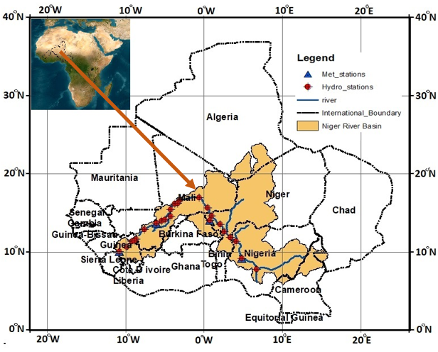
2.3. Case Study: The Niger River Basin
The Niger River Watershed, located in West Africa between latitudes 4°10′ N and 23°57′ N, and longitudes 11°50′ W and 15°48′ E, encompasses a vast catchment area of approximately 2.156 million km
2, making it the ninth largest in the world., The River is the third longest river in Africa, spanning a distance of 4200 km, coursing through over 10 countries, including Benin, Algeria, Burkina Faso, Chad, Cameroon, Côte d’Ivoire, Mali, Guinea, Niger, and Nigeria (see
). The climate within the Niger River Watershed is characterized by its complexity, with distinct variations in precipitation patterns along a north-south axis.
. Niger River Basin, with its distribution of the climatic and hydrological stations.
This region is influenced by the tropical convergence zone, resulting in well-defined dry (October to June) and wet seasons (July to September). According to [
44], West Africa (WA) is experiencing rapid growth in comparison to other regions on the African continent. This growth may be ascribed to the creation and growth of the Economic Community of West African States, which has resulted in an increase in the population of the region (with a mean annual growth rate of 7%) and a rising level of urbanization. Despite this, agriculture continues to dominate the region’s industrial sector. The agricultural production, mainly focusing on grains, livestock, and grazing [
45], contributes to 40% of the NRW’s GDP. However, due to the expanding human presence, the water security of the watershed is facing significant challenges [
46]. The watershed has a total of 26 hydrological gauge stations spread across five countries, namely Guinea, Mali, Niger, Nigeria, and Burkina Faso, as seen in
.
However, it is critical to emphasise that the 26 stations have a significant quantity of missing data, which leads to incorrect time series observations. A review of data consistency and trends revealed inconsistencies across all the stations. Therefore, we conducted a detrending inquiry using a moving average approach for only one station [
47]. As a result, the chosen station’s detrend data (Niamey) spans 30 years, from 1993 to 2022. This is due to the previously specified constraint.
2.4. Time Lag Scenarios on Climate Data
This study evaluated model sensitivity using three input scenarios (
). The default inputs, referred to as S1, were daily mean precipitation, maximum temperature (max
temp), and minimum temperature (min
temp) from the selected hydrological station and appropriately captured the average climatic conditions of the study area. We use these inputs to drive the hybrid models of the MLs. In the next input scenario S2, focused on integrating lagged rainfall, min
temp, and streamflow data. The lagging of the input data is based on the cross-correlation and partial autocorrelation function (PACF) analyses utilised by Weiß, et al. [
48] and defined, respectively, as follows:
where
n is the number of data points,
Xt and
Yt are the values of
X and
Y at time
t, $$\overset{-}{X}$$ and $$\overset{-}{Y} $$are the means of
X and
Y, respectively.
. A statistical description of the climate data and their Partial Autocorrelation plots.
The PACF of a time series
X at
lag k, denoted as
ϕkk, is the correlation between
Xt and
Xt−k that is not accounted for by
lags 1 through
k − 1. It can be calculated using the Yule-Walker equations for an autoregressive (AR) process of order
k:
where
γ(
k) is the autocovariance at lag
k and
γ(0) is the variance of the time series. Using this method, further scenarios were created and referred to as forcing data. This data aids in accurately representing the hydrological response of the watershed and the direction of streamflow during model training. At hydrological stations, the measured rainfall, min
temp, and max
temp are represented by S1.
summarises the S3 and S4 scenarios that arise from the inclusion of the lagged rainfall, min
temp, and streamflow in S2.
.
Input Scenarios for the Prediction of Streamflow using SVM hybrid models.
| Daily Lags |
Significant Cross-Correlation Coefficients from PACF |
Scenarios |
Scenarios Description |
Additional Features |
Rational |
| Mali Station |
Niger Station |
Lokoja Station |
| 1 |
1.00 |
1.00 |
1.00 |
S1 |
Rainfall, MinTemp, Maxtemp, streamflow |
|
Basic setup with daily mean rainfall, maximum temperature and minimum temperature and stemflows |
| 2 |
−0.72 |
−0.84 |
−0.90 |
S2 |
Rainfall, Mintemp, Maxtemp, Lagged Rainfall, Lagged Mintemp+ Streamflow |
Lagged rainfall (one-day lag), Lagged Mintemp (one-day lag), Lagged streamflow |
Builds upon S1 by Adding Lagged rainfall, minimum temperature, and streamflow based on significant lags |
| 3 |
0.30 |
−0.36 |
−0.57 |
S3 |
Rainfall, Mintemp, Maxtemp, Lagged Rainfall, Lagged Mintemp, Lagged streamflow |
Lagged rainfall (two-day lag), Lagged Mintemp (two-day lag), Lagged streamflow |
Extends S2 by adding lagged streamflow based on significant lags observed in partial autocorrelation analysis |
| 4 |
−0.13 |
−0.16 |
−0.88 |
S4 |
Rainfall, Mintemp, Maxtemp, Lagged Rainfall, Lagged Mintemp, Lagged streamflow |
Lagged rainfall (three-day lag), Lagged Mintemp (three-day lag), Lagged streamflow |
Extends S3 by adding lagged streamflow based on significant lags observed in partial autocorrelation analysis |
The adoption of a differencing standardisation approach was employed in order to achieve meaningful comparison, enhance model performance, and reduce outliers in the time series data at the same time, ensuring peak flows are well captured in the prediction. This approach makes data stationary and simpler to analyse since statistical features like mean and variance do not vary. Further, this type of evaluation becomes useful in the context of streamflow forecasting. The standardization process of differencing comprises the calculation of the divergence between successive observations within the time series. Mathematically, differencing can be expressed as:
where Δ
Xt is the differenced value at time
t,
Xt is the original value at time
t, and X
t−1 is the original value at time
t − 1.
The imputation methods used in this study were primarily linear interpolation and multiple imputations (MI), depending on the nature and extent of missing data within the time series. Since streamflow and meteorological variables (rainfall, min
temp, max
temp) exhibit strong temporal autocorrelation (
), linear interpolation preserves the underlying trend without introducing significant bias. While on the other hand, MI improves robustness, especially when missing data is not completely random (e.g., seasonal patterns in rainfall and streamflow). It prevents underestimation of variability that often occurs with single imputations like mean or median filling.
In this study, to ensure effective computation, the data is split from 1 January 1993 to 31 December 2011 for model training and data from 1 January 2012 to 30 December 2022 for testing considering threefold Cross-validation (CV) (
k = 3).
2.5. Hyperparameter Optimization Strategy
To optimize the hyperparameters of the Support Vector Regression (SVR) model, four metaheuristic algorithms—BSMA, AVOA, AA, and IIFA—were employed. The optimization process aimed to enhance SVR’s predictive performance by fine-tuning three key hyperparameters: the regularization parameter (C), which controls the trade-off between model complexity and training error; the tube radius (Epsilon), which defines the margin of tolerance for prediction errors; and the kernel coefficient (Gamma), which determines the influence of individual training examples in the radial basis function (RBF) kernel. The search space for these hyperparameters was predefined based on empirical testing and prior studies to ensure a balance between exploration and computational efficiency. The objective function for the optimization was to minimize the Mean Absolute Error (MAE) between observed and predicted streamflow values. Each algorithm iteratively adjusted the SVR hyperparameters to reduce MAE, following its unique search mechanism.
A consistent train-test split was used across all models to ensure a fair comparison. To validate the optimized hyperparameters,
k-Fold Cross-Validation (
k = 5) was employed, reducing the risk of overfitting and ensuring robust model generalization. The final hyperparameter values obtained for each algorithm across different prediction scenarios (S1–S4) are presented in
, demonstrating how each optimization method influenced the SVR model’s configuration. By systematically tuning the SVR hyperparameters, this methodology ensures an effective and unbiased comparison of metaheuristic-based optimization strategies for streamflow prediction.
.
Hyperparameter distribution of SVR model determine under each Meta-heuristic Algorithms.
| Prediction Scenarios |
BSMA |
AVOA |
AA |
IIFA |
| C |
Epsilon |
Gamma |
C |
Epsilon |
Gamma |
C |
Epsilon |
Gamma |
C |
Epsilon |
Gamma |
| S1 |
10 |
0.8 |
0.1 |
16.66 |
0.01 |
0.1 |
1000 |
0.01 |
0.00091 |
267 |
0.405 |
0.0021 |
| S2 |
10 |
0.36 |
0.1 |
15.4 |
0.01 |
0.1 |
1000 |
0.132 |
0.1 |
241 |
0.178 |
0.0016 |
| S3 |
10 |
0.02 |
0.1 |
57.71 |
0.01 |
0.1 |
1000 |
0.185 |
0.1 |
197 |
0.316 |
0.001 |
| S4 |
10 |
0.14 |
0.1 |
65.27 |
0.5 |
0.0001 |
1000 |
0.199 |
0.1 |
191 |
0.312 |
0.001 |
3. Results and Discussion
3.1. Optimised Hyperparameters for SVM Models
provides a detailed analysis of the distribution of the Support Vector Regression (SVR) model’s hyperparameters when utilising various metaheuristic methods for prediction. We looked at three hyperparameters—Regularisation Parameter (C), Tube Radius (epsilon), and Kernel Coefficient (gamma)—that have a significant effect on how well the SVR model predicts streamflow. When compared to other algorithms, BSMA tends to pick smaller numbers for C and Epsilon. In S1, BSMA picks out C to be equal to 10, Epsilon is equal to 0.8, and Gamma is equal to 0.1. In S2, C = 10, Epsilon = 0.36, and Gamma = 0.1 mean the following things: Specifically, the numbers given for S3 are C = 10, Epsilon = 0.02, and Gamma = 0.1. The BSMA method picks the numbers C = 10, Epsilon = 0.14, and Gamma = 0.1 for S4. When it comes to regularisation (C) and margin error (Epsilon), BSMA pick smaller numbers, which allow the model to find a simpler decision function, which may improve generalisation to unseen data. At the same time, the large epsilon values for S1, S2, and S4 allow more errors within the margin, resulting in a simpler model as compared to S3, which will allow the model to be more sensitive to errors, potentially leading to a more complex model.
AVOA, on the other hand, tends to pick higher values for parameter C and smaller values for parameter Epsilon. When it comes to S1, AVOA optimised the C value at 16.66, Epsilon to be 0.01, and Gamma as 0.1, which is similar to S2, except for the C value, which is 15.4. For S3, AVOA chooses C = 57.71 with the same Epsilon and Gamma values, whereas for S4, the C value is 65.27, Epsilon is 0.5, and Gamma is 0.0001. As you can see from these numbers (), AVOA tends to support higher levels of regularisation (C) and lower levels of margin error (Epsilon). This lets the model fit the training data more closely, which could lead to overfitting. On the other hand, this can make the decision boundary smooth. In each case, AA always picks high numbers for C (C = 1000), as shown in S1, S2, S3, and S4, while also varying Epsilon and Gamma from 0.01 to 0.199 and 0.00091 to 0.1, respectively. The results show that AA has a strong tendency towards high regularisation (C), which allows it to control the trade-off between achieving a low error on the training data and minimising the complexity of the decision function.
.
Performance evaluation across meta-heuristic algorithms for each scenario.
| Scenarios |
Meta-Heuristic Algorithms |
Performance Matric |
| ARE |
C |
P |
RMSE |
NSE |
MAE |
R2 |
| S1 |
BSMA |
1.818 |
0.965 |
0.855 |
0.766 |
0.965 |
7.318 |
0.986 |
| S2 |
2.227 |
0.966 |
0.825 |
1.004 |
0.944 |
9.199 |
0.976 |
| S3 |
2.428 |
0.960 |
0.815 |
1.088 |
0.912 |
10.135 |
0.972 |
| S4 |
2.698 |
0.956 |
0.806 |
1.119 |
0.863 |
10.755 |
0.970 |
| S1 |
AVOA |
1.662 |
0.999 |
0.863 |
0.736 |
0.999 |
6.911 |
0.987 |
| S2 |
1.696 |
0.975 |
0.855 |
0.900 |
0.971 |
7.878 |
0.981 |
| S3 |
3.380 |
0.942 |
0.775 |
1.265 |
0.942 |
12.537 |
0.962 |
| S4 |
12.253 |
0.848 |
0.479 |
2.599 |
0.524 |
44.847 |
0.839 |
| S1 |
AA |
4.420 |
0.051 |
0.041 |
0.010 |
0.999 |
0.199 |
0.995 |
| S2 |
3.562 |
0.044 |
0.031 |
0.010 |
0.986 |
0.199 |
0.996 |
| S3 |
3.217 |
0.043 |
0.029 |
0.010 |
0.999 |
0.199 |
0.996 |
| S4 |
3.032 |
0.012 |
0.017 |
0.010 |
0.988 |
0.199 |
0.996 |
| S1 |
IIFA |
0.061 |
0.042 |
0.999 |
4.391 |
0.985 |
4.197 |
0.995 |
| S2 |
1.130 |
0.981 |
0.894 |
0.651 |
0.973 |
6.748 |
0.989 |
| S3 |
0.760 |
0.998 |
0.917 |
0.575 |
0.952 |
5.290 |
0.992 |
| S4 |
0.749 |
0.999 |
0.920 |
0.566 |
0.893 |
5.227 |
0.992 |
In the end, compared to other algorithms, the IIFA algorithm usually picks moderate numbers for both C and small numbers for Epsilon. In the given scenario, IIFA sets different values for C, Epsilon, and Gamma for four different scenarios (S1 to S4). For example, in S1, IIFA sets C = 100, Epsilon = 10, and Gamma = 0.01. These values determine the trade-off between model complexity and training error, the influence of individual training examples, and the margin of tolerance for errors, respectively. Generally, large C values (e.g., C > 100) indicate a more complex model; small epsilon values (e.g., Epsilon < 0.1) increase sensitivity to errors; and small gamma values (e.g., Gamma < 0.01) lead to smoother decision boundaries. Because of this, each metaheuristic algorithm has a unique tendency towards certain hyperparameter values, which shows how they optimise problems. For the SVR model to work at its best, it is important to pick the right hyperparameters. The results show how important it is to look into different metaheuristic algorithms to find the ones with the best choices for a certain prediction case.
3.2. Results of All the Cases Considered in Streamflow Time Series Predictions
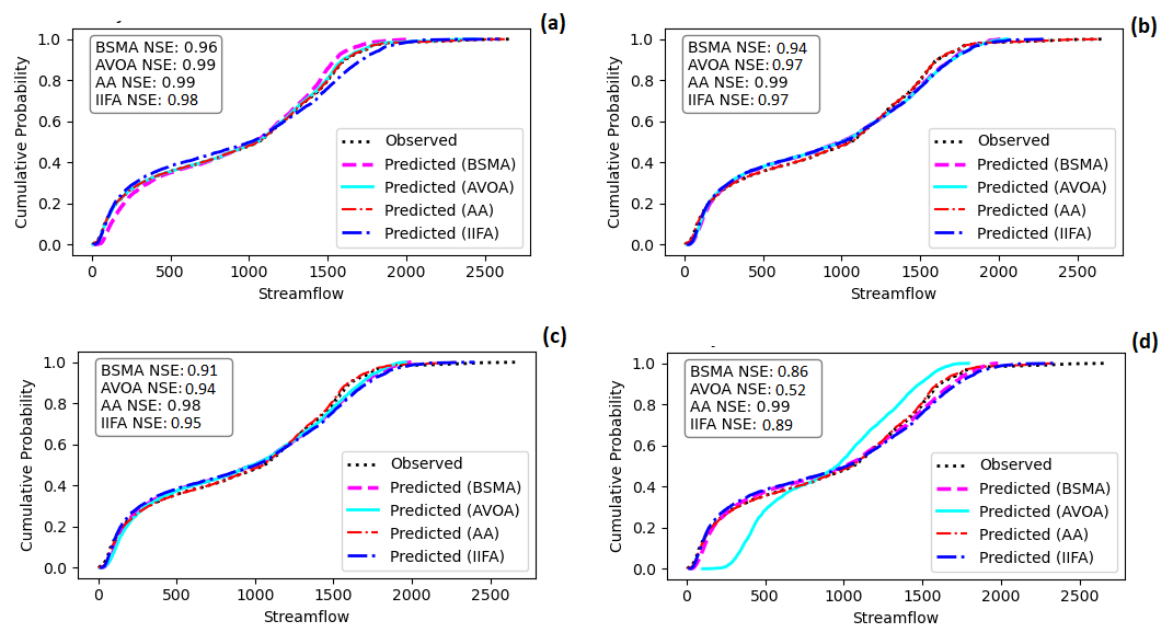
In scenario-S1, the SVM-BSMA achieves a Nash-Sutcliffe Efficiency (NSE) of 0.965, demonstrating a robust correlation between the observed and predicted daily streamflows. The cumulative probability curve aligns with the 1:1 line, indicating that the model accurately captures streamflow range and pattern. SVM-AVOA surpasses BSMA with an NSE of 0.999, and the cumulative probability curve matches the 1:1 line, demonstrating a good match between projected and observed streamflows. The SVM-AA model, with an NSE of 0.999, provides accurate streamflow predictions in S1, similar to the SVM-AVOA model. In Scenario-S1, the SVM-IIFA has an NSE of 0.985, which is lower than the SVM-AA and SVM-BSMA hybrid models. In essence, SVM-IIFA has a lower cumulative probability curve than SVM-AA and SVM-AVOA, but it matches the predicted and observed streamflows. The SVM-BSMA performs well in Scenario-S2, with an NSE of 0.9441. The cumulative probability curve would match the 1:1 line, indicating a strong correlation between predicted and observed streamflows. With an NSE of 0.971, SVM-AVOA does a good job in this case. The model’s cumulative probability curve is very close to the 1:1 line (
b), which means that predicted and observed values are very close to each other. With an NSE value of 0.986, the SVM-AA model also does well in Scenario 2 because its cumulative probability curve crosses the 1:1 line, meaning that expected and observed streamflows are very similar. In S2, the SVM-IIFA model performs well, with an NSE of 0.973, and it matches the forecast and observed streamflows, though less than SVM-AA.
. The NSE CDFs of BSMA, AVOA, AA, and IIFA for each Scenario (<b>a</b>) S1 (<b>b</b>) S2 (<b>c</b>) S3 and (<b>d</b>) S4.
In scenario S3, the SVM-BSMA works well with an NSE of 0.9119, and the cumulative probability curve’s departure from the 1:1 line shows that the expected and observed streamflows are not the same. But, the SVM-AVOA model performs well, with an NSE of 0.942 and good fits between projected and actual streamflows. However, SVM-AA shows excellent performance, with an NSE score of 0.999 and close to a 1:1 line, indicating exceptional performance. When compared to the observed data, SVM-IIFA prediction performance under S3 yielded an NSE value of 0.952. The cumulative probability curve matches forecast and observed streamflows, albeit less than SVM-AA (c).
In Scenario-S4 (d), the SVM-BSMA performs well, with an NSE value of 0.8634. This differs from the 1:1 line in the cumulative probability curve, meaning that the predicted and observed streamflows don’t match up. SVM-AVOA does not do well in S4 (NSE score of 0.524), and the cumulative probability curve is very far from the 1:1 line, showing a big difference between what was predicted and what was observed in terms of streamflows. Although SVM-AA has an NSE value of 0.9876, this makes a good prediction in S4, as the cumulative probability curve for SVM-AA is close to 1:1. With an NSE of 0.893, the SVM-IIFA excels in S4, closely matching the projected and actual streamflows. As shown by using NSE values to describe how well models predict streamflows, the details make it easy to understand how well the hybrid model worked (d). The cumulative probability curve also helps to see how well it worked.
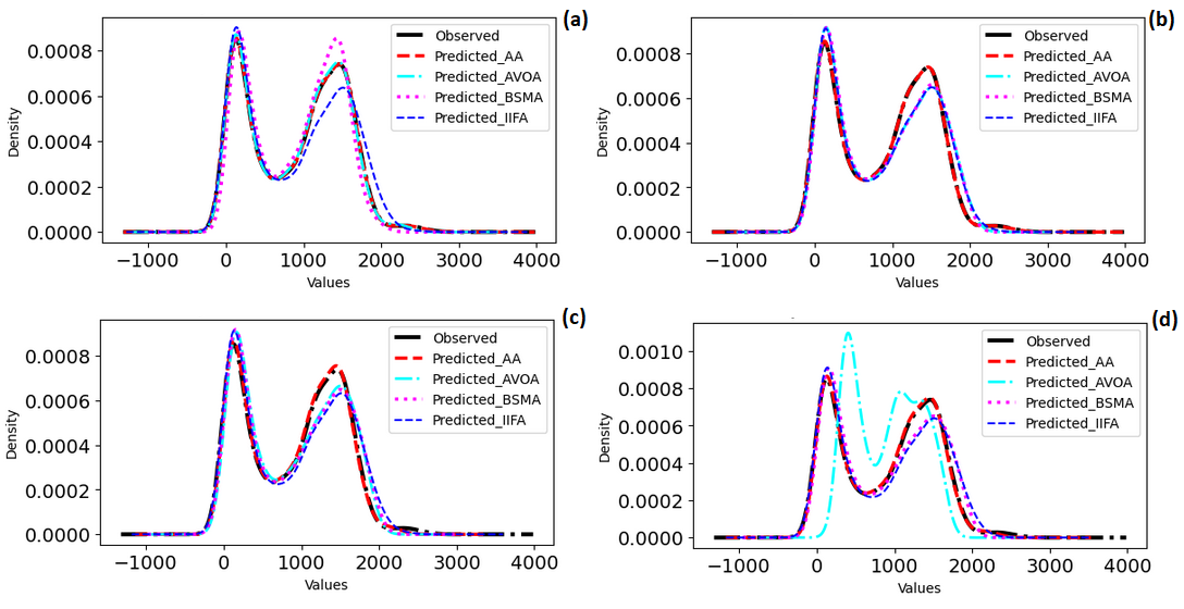
A density map was generated to assess the hybrid models’ predictive capability in capturing the temporal fluctuations of streamflows under high and low flow conditions (a–d). It is employed to depict the distribution of a continuous variable by generating a continuous probability density function that accurately matches the data and illustrates the relative probability of different values appearing in the data. During high flows, all the models successfully replicated the phenomenon in all four scenarios. However, the effect was more noticeable in scenarios S1, S2, and S3 but diminished in scenario S4. However, after analysing the high flows at the 75th percentile, it was noted that the performance of the hybrid models differed across the four scenarios. The SVM-AA model accurately captures the peak flow range, followed by the SVM-BSMA model. The SVM-IIFA model performs somewhat worse, and the SVM-AVOA model performs the least well, as shown in a,d. Regarding the prediction of low flow, all models demonstrate good performance, except for SVM-BSMA, which notably forecasts larger low flows compared to the other models (refer to c,d). When considering settings where the flow is decreasing, SVM-AA outperforms SVM-BSMA, SVM-IIFA, and SVM-AVOA in capturing the flow. This conclusion is based on their performance in different scenarios, as shown in a–d.
. A density plots of the predicted and observed Streamflow under (<b>a</b>) S1 (<b>b</b>) S2 (<b>c</b>) S3 (<b>d</b>) S4.
Metaheuristic algorithms, inspired by natural processes, solve many complex optimisation issues [
49]. However, in order to optimise the target parameter and guarantee reliable prediction, every method has a distinct impact. Therefore, we created standard criteria for the target hyperparameters, performance assessment, and computational procedure. We subjected all hybrid models to a maximum of 100 iterations throughout the computational process, and used an 8-performance matrix to assess their influence on improving the SVR model for accurate daily streamflow prediction. provides a comprehensive analysis of the hybrid models’ performance in various scenarios. Every scenario denotes a distinct combination of parameters or degrees of intricacy for the optimisation problem. These measures aid in gauging the performance of the algorithms in terms of accuracy, convergence speed, and data fit. Its result indicates that SVM-BSMA does well in Scenario S1, with a posterior error ratio (C) of 0.855, an absolute relative error (ARE) of 1.818, and a small error probability (P) of 0.965. Nevertheless, its root means square error (RMSE) and mean absolute error (MAE) values exhibit a slight rise when compared to other methods in S1. Even so, SVM-BSMA does very well in terms of NSE (Nash-Sutcliffe Efficiency) and
R2 (coefficient of determination), which means it does very well overall in S1. In subsequent scenarios (S2, S3 and S4), the SVM-BSMA model performance experiences a minor drop, characterized by higher absolute relative error (ARE) values and reduced precision. However, it still retains a tolerable small error probability (P) and posterior error ratio (C).
The SVM-AVOA model has strong performance in S1, achieving an ARE of 1.662 and a P of 0.999. In Scenario-S4, however, SVM-AVOA’s performance drops a lot, as shown by an ARE of 12.253 and a P of 0.848. This suggests that SVM-AVOA may encounter difficulties when dealing with intricate or noisy data [
50]. SVM-AVOA exhibits varying performance in different settings, demonstrating satisfactory accuracy in simpler situations but inadequate performance in more intricate ones. In all cases, SVM-AA’s performance is consistently subpar for ARE values ranging from 3.032 to 4.420 and an extremely low small error probability (P) of less than 0.1. On the other hand, other tests (RMSE, NSE, MAE, and R2) have shown that SVM-AA has done really well. This means that it is a good choice for the optimisation tasks we looked at because it gives accurate and consistent results in many situations. The SVM-IIFA model performs well in all scenarios, with an average relative error (ARE) ranging from 0.612 to 1.130 and an accuracy above 0.97 in the majority of cases. In addition, the model has a small likelihood of P and a favourable ratio of posterior errors (C), as evidenced by its RMSE, NSE, MAE, and
R2 values. These findings suggest that IIFA is a reliable and efficient metaheuristic algorithm for the optimisation tasks examined in the present study.
A critical aspect influencing the reliability of the hybrid SVR models is the selection of time lags in streamflow prediction (S1 to S4). To quantify this impact, we conducted a statistical analysis comparing different lag structures (e.g., 1-day, 2-day, 3-day lags) on key model performance metrics such as RMSE, NSE, and ARE. The findings indicate that while shorter lags (1-day) provide higher accuracy in capturing immediate fluctuations, longer lags (3-day) tend to introduce higher errors due to increased uncertainty in hydrological response. For instance, in Scenario S1, SVM-BSMA exhibited an NSE of 0.965 with a 1-day lag but dropped to 0.912 with a 3-day lag. Similarly, SVM-AVOA’s ARE increased significantly from 1.662 to 3.380 when transitioning from a 1-day to a 3-day lag, indicating reduced predictive efficiency in longer forecasting windows. These results demonstrate the need for careful lag selection when optimizing streamflow predictions, particularly in basins with varying hydrological regimes.
To assess the broader applicability of the proposed models, future research should consider transfer learning approaches, where models trained in one basin are fine-tuned using limited data from another basin. This technique can help determine the extent to which the optimized models retain predictive skills in new environments. Additionally, comparative studies across multiple basins with contrasting hydrological conditions would provide valuable insights into how metaheuristic algorithms perform across different settings.
Despite these limitations, the study provides a strong foundation for optimizing machine learning models in streamflow prediction, particularly in data-scarce environments like West Africa. By incorporating adaptive modeling techniques and additional calibration strategies, the proposed hybrid models could be extended to other regions with different climatic and hydrological characteristics.
3.4. Analysis of the Results
Particularly in dynamic and complicated contexts like time series prediction, metaheuristic algorithms are potent tools for optimising hyperparameters in machine learning models [
51]. Using a variety of performance metrics, we compare four different metaheuristic algorithms—BSMA, AVOA, AA, and IIFA—across four different scenarios to find the optimal method for choosing metaheuristic algorithms to optimise the hyperparameters of machine learning models used in time series prediction. One way to learn about the optimisation tendencies of different algorithms is to look at their hyperparameter distributions [
52]. In order to promote simpler decision functions and maybe greater generalisation to unseen data, BSMA prefers to use smaller values for the Regularisation Parameter (C) and Tube Radius (Epsilon).
Conversely, AVOA has a tendency to pick lower Epsilon values and larger C values, which might bring the model closer to the training data but also raise the possibility of overfitting. The fact that AA always goes with large values for C suggests that it prefers to manage the trade-off between a small decision function and no training mistake [
53]. In order to strike a compromise between the complexity of the model and the training error, IIFA typically uses modest values for Epsilon and C. To give a full picture of each method, we added the performance evaluation across several circumstances. For instance, it showed that IIFA maintained superior performance over the other algorithms in all cases, with lower ARE values and better accuracy (). In less complicated circumstances, BSMA performed competitively, but in more difficult ones, it somewhat underperformed. Perhaps as a result of overfitting, AVOA fared poorly in more complicated scenarios despite doing admirably in simpler ones.
The fact that AA outperformed some other algorithms shows that it is well-suited to the optimisation tasks under consideration. Since IIFA consistently performs well in all of the tested circumstances, it stands out as a potential choice in our research. Nevertheless, meticulous assessment of the algorithms employing a mix of performance indicators and sophisticated selection criteria should underpin the selection process [
54]. Model complexity, generalisability, and computing efficiency are all trade-offs that should be considered while choosing the optimal metaheuristic method for hyperparameter optimisation [
55,
56]. Still, for optimising hyperparameters in machine learning models for time series prediction, the study sheds light on how metaheuristic algorithms fare. In order to choose the best algorithm for a certain problem, it is crucial to take into account both basic selection criteria and performance measures [
50]. The consistency of performance across circumstances makes IIFA a potential candidate, followed by AA, BSMA, and then AVOA. Nevertheless, meticulous assessment of the algorithms employing a mix of performance indicators and sophisticated selection criteria should underpin the selection process [
57].
However, streamflows are complex natural phenomena that change as environmental factors vary [
58], but the ability of the MLs to capture this uniqueness required several amalgamations of the MAs to adequately capture this complex behaviour, which this study intends to showcase. In West Africa, we expect streamflow in large rivers such as the Niger River Basin, spanning several thousand kilometres, to traverse diverse climate zones, each contributing differently to the streamflow behaviour. These hybrid models’ ability to capture this complexity with such accuracy is a testament to their reliability in mimicking natural processes.
One crucial aspect that requires further exploration is the impact of time lag on model performance. The choice of time lag significantly influences the predictive accuracy and generalizability of time series models. In hydrological modeling, streamflow responses to rainfall or other climatic variables are often delayed, meaning that selecting an optimal lag period is essential for capturing the relationship between past and present observations [
59]. Different lag scenarios may lead to variations in model performance, where a short lag might fail to account for delayed responses in the system, while an excessively long lag could introduce unnecessary noise, reducing the model’s predictive capability.
Metaheuristic algorithms optimize hyperparameters, but their effectiveness may vary depending on how well they handle time-dependent features [
60]. For instance, algorithms like BSMA and IIFA, which tend to balance complexity and accuracy, may be better suited to selecting appropriate lag structures that enhance model generalizability. Conversely, AVOA’s tendency toward overfitting suggests that it may struggle with lag selection, as it may focus too closely on recent observations while neglecting longer-term dependencies [
61]. Similarly, AA, which prioritizes minimizing training error, might require additional tuning to handle lag effects effectively.
It is important to note that despite interpretability methods such as SHAP and LIME providing insights into feature contributions, they were not employed in this study due to the focus on optimizing model accuracy and generalization rather than feature attribution. Instead, we relied on direct performance evaluation metrics (e.g., NSE, RMSE, MAE, and R²) and comparative analysis across multiple scenarios to validate model reliability. Future work can incorporate interpretability techniques to enhance model transparency where necessary further.
To improve model reliability, future research should investigate optimal time lag determination strategies, particularly within metaheuristic-based optimization frameworks. This could involve adaptive lag selection techniques that dynamically adjust based on changing hydrological conditions. Furthermore, the interaction between lag choice and model complexity should be examined to determine how different metaheuristic algorithms respond to varying lag structures and whether certain algorithms exhibit greater robustness to lag-induced variability in time series prediction.
Another critical consideration is how missing and inconsistent hydrological data were handled and the potential impact of data gaps on model performance. While data availability issues in the Niger River Basin have been acknowledged, the preprocessing steps taken to address these gaps require further clarification. Missing data in hydrological records can arise due to instrument failure, human errors, or extreme weather conditions, which can introduce bias and reduce model reliability [
62]. To mitigate these challenges, a combination of imputation techniques and data filtering methods was employed. Specifically, linear interpolation and multiple imputation approaches were used to estimate missing values where gaps were relatively short, while longer gaps were addressed using machine learning-based imputation techniques [
63]. These techniques helped preserve data continuity and minimize distortions in the streamflow time series.
The impact of missing data on model performance varies depending on the extent and distribution of the gaps. In cases where missing values were randomly distributed, the effect on predictive accuracy was minimal [
64]. However, systematic gaps, particularly those occurring during peak flow or dry season, could lead to biases in model training, as key hydrological patterns might be underrepresented. To account for this, sensitivity analyses were conducted to evaluate model performance under different missing data scenarios, as detailed by Fawkes, et al. [
65] and Baig, et al. [
66]. The results indicated that models trained with imputed datasets performed comparably to those trained on complete datasets, provided that imputation methods were carefully selected based on the data distribution [
67].
It is well-known fact that the Hydrological modeling is highly dependent on regional characteristics such as topography, land use, climate variability, and basin-scale hydrodynamics. These factors influence how well a model trained in one region can be applied to another with distinct environmental conditions [
68]. The Niger River Basin is characterized by diverse climatic zones, ranging from humid regions in the south to arid and semi-arid conditions in the north. This inherent variability suggests that the proposed hybrid models can handle a broad range of hydrological conditions within the basin itself. However, how do these unique characteristics of the Niger River Basin impact the model’s performance in other regions? The complex interplay between climatic zones means that models optimized for this basin may require significant recalibration when applied to areas with different precipitation patterns, soil types, and hydrological processes. For instance, while the Niger Basin experiences both seasonal flooding and prolonged dry periods, basins dominated by snowmelt or monsoonal rainfall would need modifications to account for delayed runoff or extreme seasonal fluctuations. Applying these models to other river basins—such as those in temperate or monsoonal regions—may introduce new challenges related to data availability, rainfall-runoff relationships, and seasonality effects.
One key factor influencing generalizability is the ability of metaheuristic algorithms to adapt to different hydroclimatic conditions [
31]. Algorithms like IIFA and BSMA, which balance complexity and accuracy, may be more flexible across regions with varying rainfall patterns, soil characteristics, and land cover dynamics. Conversely, AVOA’s tendency toward overfitting suggests that it might struggle when applied to basins with significantly different hydrological regimes, requiring additional tuning to avoid model bias. Another important consideration is the role of extreme hydrological events. Some basins experience more frequent or intense floods and droughts, which can impact the performance of machine learning models [
69]. For instance, regions prone to flash floods, such as mountainous basins, may require models that incorporate higher-resolution rainfall data and terrain-sensitive hydrological parameters. Similarly, basins dominated by snowmelt processes would need additional modifications to account for delayed runoff generation due to seasonal temperature variations.
Our findings align with previous research in demonstrating the effectiveness of metaheuristic algorithms for optimizing SVM-based streamflow prediction models. For instance, studies such as Sharma and Raju [
49] and Pham, et al. [
50] highlight the ability of hybrid models to improve predictive accuracy. However, our results show notable differences in algorithm performance under varying hydrological conditions. Unlike prior studies that primarily focused on specific climatic regions, our analysis incorporates diverse hydroclimatic scenarios, revealing that SVM-BSMA and SVM-IIFA exhibit greater adaptability across different rainfall-runoff dynamics. In contrast, SVM-AVOA’s performance declines significantly in more complex scenarios, suggesting a potential limitation in handling intricate or noisy datasets. These divergences likely stem from differences in methodology—particularly in hyperparameter tuning constraints and iteration limits—as well as variations in dataset characteristics, including temporal resolution and regional hydrological variability. Future comparative studies should further investigate these factors to enhance model robustness and transferability across diverse basins.
The findings of this study have significant implications for water resource management, policy development, and community adaptation strategies in the Niger River Basin. Given the increasing variability in streamflow patterns, it is essential to integrate actionable measures that bridge the gap between research and real-world applications. Effective flood mitigation strategies, water allocation planning, and adaptive management approaches could benefit from the insights provided by optimized machine learning models [
70]. By improving predictive accuracy, these models can enhance early warning systems and support decision-making for sustainable water use.
Furthermore, the impact of climate change on streamflow variability warrants deeper consideration. Changing precipitation patterns and rising temperatures have the potential to alter hydrological cycles, disrupt water availability, and degrade water quality [
71,
72]. These shifts pose challenges for long-term water security, particularly in transboundary river basins like the Niger River Basin, where competing demands for water resources necessitate robust management frameworks. Integrating climate change projections into hydrological modeling efforts could strengthen the study’s applicability in addressing future water scarcity and flood risks.
4. Conclusions
For the purpose of optimising the hyperparameters of the support vector machine (regressor) used to forecast streamflow in hydrology, this study compared the efficiency of four metaheuristic algorithms: the Binary Slime Mould Algorithm (BSMA), the African Vulture Optimisation Algorithm (AVOA), the Archery Algorithm (AA), and the Intelligent Ice Fishing Algorithm (IIFA). The study’s findings shed light on each algorithm’s optimisation approaches and generalisability. The findings show that different algorithms have different preferences when it comes to the values of the hyperparameters, which can have a major effect on how well the SVM model works. Overall, the results show that:
- i.
-
BSMA preferred simpler decision functions; AVOA preferred closer fits to training data; AA preferred controlling the complexity-error trade-off; and IIFA sought a balance between the two.
- ii.
-
IIFA and AA consistently outperformed the other algorithms across different scenarios, proving their effectiveness in optimising hyperparameters for SVR models in time series prediction.
- iii.
-
Hybrid techniques integrating several metaheuristic algorithms could be the subject of future research if we want to improve optimisation performance even further in complicated machine learning problems.
Acknowledgments
The authors acknowledge support from the Department of Water Resources and Environmental Engineering, Ahmadu Bello University, Zaria, Nigeria.
Author Contributions
A.-A.D.B.: Conceptualization, Methodology, software, writing—original draft; B.U.A. Writing—validation, review, and editing; A.S: Visualization and editing; B.T.: writing—Data curation and editing; K.S: writing—review and editing; A.I.: writing—review and editing. All authors have read and agreed to the published version of the manuscript.
Ethics Statement
Not applicable.
Informed Consent Statement
Not applicable.
Data Availability Statement
Original data and code are available from the corresponding author upon reasonable request.
Funding
This research received no external funding.
Declaration of Competing Interest
The authors declare no conflicts of interest.
References
1.
Papa F, Crétaux JF, Grippa M, Robert E, Trigg M, Tshimanga RM, et al. Water resources in Africa under global change: monitoring surface waters from space.
Surv. Geophys. 2023,
44, 43–93.
[Google Scholar]
2.
Tarpanelli A, Paris A, Sichangi AW, OLoughlin F, Papa F. Water resources in Africa: The role of earth observation data and hydrodynamic modeling to derive river discharge.
Surv. Geophys. 2023,
44, 97–122.
[Google Scholar]
3.
Nkiaka E, Taylor A, Dougill AJ, Antwi-Agyei P, Adefisan EA, Ahiataku MA, et al. Exploring the need for developing impact-based forecasting in West Africa.
Front. Clim. 2020,
2, 565500.
[Google Scholar]
4.
Awotwi A, Annor T, Anornu GK, Quaye-Ballard JA, Agyekum J, Ampadu B, et al. Climate change impact on streamflow in a tropical basin of Ghana, West Africa.
J. Hydrol. Reg. Stud. 2021,
34, 100805.
[Google Scholar]
5.
Larbi I, Nyamekye C, Dotse S-Q, Danso DK, Annor T, Bessah E, et al. Rainfall and temperature projections and the implications on streamflow and evapotranspiration in the near future at the Tano River Basin of Ghana.
Sci. Afr. 2022,
15, e01071.
[Google Scholar]
6.
Namugize JN, Jewitt G, Graham M. Effects of land use and land cover changes on water quality in the uMngeni river catchment, South Africa.
Phys. Chem. Earth Parts a/b/c 2018,
105, 247–264.
[Google Scholar]
7.
Djan’na Koubodana H, Adounkpe JG, Atchonouglo K, Djaman K, Larbi I, Lombo Y, et al. Modelling of streamflow before and after dam construction in the Mono River Basin in Togo-Benin, West Africa.
Int. J. River Basin Manag. 2023,
21, 265–281.
[Google Scholar]
8.
Obahoundje S, Diedhiou A, Kouassi KL, Ta MY, Mortey EM, Roudier P, et al. Analysis of hydroclimatic trends and variability and their impacts on hydropower generation in two river basins in Côte d’Ivoire (West Africa) during 1981–2017.
Environ. Res. Commun. 2022,
4, 065001.
[Google Scholar]
9.
Chun KP, Dieppois B, He Q, Sidibe M, Eden J, Paturel J-E, et al. Identifying drivers of streamflow extremes in West Africa to inform a nonstationary prediction model.
Weather. Clim. Extrem. 2021,
33, 100346.
[Google Scholar]
10.
Bjornlund V, Bjornlund H, Van Rooyen AF. Why agricultural production in sub-Saharan Africa remains low compared to the rest of the world–a historical perspective.
Int. J. Water Resour. Dev. 2020,
36, S20–S53.
[Google Scholar]
11.
Huang Z, Liu X, Sun S, Tang Y, Yuan X, Tang Q. Global assessment of future sectoral water scarcity under adaptive inner-basin water allocation measures.
Sci. Total Environ. 2021,
783, 146973.
[Google Scholar]
12.
Arsenault R, Côté P. Analysis of the effects of biases in ensemble streamflow prediction (ESP) forecasts on electricity production in hydropower reservoir management.
Hydrol. Earth Syst. Sci. 2019,
23, 2735–2750.
[Google Scholar]
13.
Zhang X, Peng Y, Xu W, Wang B. An optimal operation model for hydropower stations considering inflow forecasts with different lead-times.
Water Resour. Manag. 2019,
33, 173–188.
[Google Scholar]
14.
Ward PJ, de Ruiter MC, Mård J, Schröter K, Van Loon A, Veldkamp T, et al. The need to integrate flood and drought disaster risk reduction strategies.
Water Secur. 2020,
11, 100070.
[Google Scholar]
15.
Fahad S, Nguyen-Thi-Lan H, Nguyen-Manh D, Tran-Duc H, To-The N. Analyzing the status of multidimensional poverty of rural households by using sustainable livelihood framework: Policy implications for economic growth.
Environ. Sci. Pollut. Res. 2023,
30, 16106–16119.
[Google Scholar]
16.
Nouaceur Z, Murarescu O. Rainfall variability and trend analysis of rainfall in West Africa (Senegal, Mauritania, Burkina Faso).
Water 2020,
12, 1754.
[Google Scholar]
17.
Adnan RM, Mostafa RR, Kisi O, Yaseen ZM, Shahid S, Zounemat-Kermani M. Improving streamflow prediction using a new hybrid ELM model combined with hybrid particle swarm optimization and grey wolf optimization.
Knowl. -Based Syst. 2021,
230, 107379.
[Google Scholar]
18.
Rajwar K, Deep K, Das S. An exhaustive review of the metaheuristic algorithms for search and optimization: taxonomy, applications, and open challenges.
Artif. Intell. Rev. 2023,
56, 13187–13257.
[Google Scholar]
19.
Ibrahim KS, Huang YF, Ahmed AN, Koo CH, El-Shafie A. A review of the hybrid artificial intelligence and optimization modelling of hydrological streamflow forecasting.
Alex. Eng. J. 2022,
61, 279–303.
[Google Scholar]
20.
Khosravi K, Golkarian A, Tiefenbacher JP. Using optimized deep learning to predict daily streamflow: A comparison to common machine learning algorithms.
Water Resour. Manag. 2022,
36, 699–716.
[Google Scholar]
21.
Kumar V, Kedam N, Sharma KV, Mehta DJ, Caloiero T. Advanced machine learning techniques to improve hydrological prediction: A comparative analysis of streamflow prediction models.
Water 2023,
15, 2572.
[Google Scholar]
22.
Ferreira RG, da Silva DD, Elesbon AAA, Fernandes-Filho EI, Veloso GV, de Souza Fraga M, et al. Machine learning models for streamflow regionalization in a tropical watershed.
J. Environ. Manag. 2021,
280, 111713.
[Google Scholar]
23.
Gharib A, Davies EG. A workflow to address pitfalls and challenges in applying machine learning models to hydrology.
Adv. Water Resour. 2021,
152, 103920.
[Google Scholar]
24.
Janga Reddy M, Kumar DN. Evolutionary algorithms, swarm intelligence methods, and their applications in water resources engineering: A state-of-the-art review.
h2oj 2020,
3, 135–188.
[Google Scholar]
25.
Tao H, Abba SI, Al-Areeq AM, Tangang F, Samantaray S, Sahoo A, et al. Hybridized artificial intelligence models with nature-inspired algorithms for river flow modeling: A comprehensive review, assessment, and possible future research directions.
Eng. Appl. Artif. Intell. 2024,
129, 107559.
[Google Scholar]
26.
Tian D, Li B, Liu J, Liu C, Yuan L, Shi Z. Adaptive Multi-Updating Strategy Based Particle Swarm Optimization.
Intell. Autom. Soft Comput. 2023,
37, 2783.
[Google Scholar]
27.
Vie A, Kleinnijenhuis AM, Farmer DJ. Qualities, challenges and future of genetic algorithms: A literature review.
arXiv 2020, arXiv:2011.05277.
[Google Scholar]
28.
Faris H, Aljarah I, Al-Betar MA, Mirjalili S. Grey wolf optimizer: a review of recent variants and applications.
Neural Comput. Appl. 2018,
30, 413–435.
[Google Scholar]
29.
Gontara E, Chebana F. Mixture copula parameter estimation with metaheuristic algorithms, comparative study under hydrological context.
Stoch. Environ. Res. Risk Assess. 2025, 1–20. doi:10.1007/s00477-025-02914-4.
[Google Scholar]
30.
Rahimzad M, Nia AM, Zolfonoon H, Soltani J, Mehr AD, Kwon H-H. Performance comparison of an LSTM-based deep learning model versus conventional machine learning algorithms for streamflow forecasting.
Water Resour. Manag. 2021,
35, 4167–4187.
[Google Scholar]
31.
Adnan RM, Mirboluki A, Mehraein M, Malik A, Heddam S, Kisi O. Improved prediction of monthly streamflow in a mountainous region by Metaheuristic-Enhanced deep learning and machine learning models using hydroclimatic data.
Theor. Appl. Climatol. 2023,
155, 205–228.
[Google Scholar]
32.
Bahramifar A, Afshin H, Tabrizi ME. Optimized simulation of river flow rate using regression-based models.
Acta Geophys. 2023,
71, 2481–2496.
[Google Scholar]
33.
Xu Y, Zomer S, Brereton RG. Support vector machines: A recent method for classification in chemometrics.
Crit. Rev. Anal. Chem. 2006,
36, 177–188.
[Google Scholar]
34.
Rieck K, Sonnenburg S, Mika S, Schäfer C, Laskov P, Tax D, et al. Support vector machines. In Handbook of Computational Statistics; Springer: New York, USA, 2012; pp. 883–926.
35.
Montesinos López OA, López AM, Crossa J. Support vector machines and support vector regression. In Multivariate Statistical Machine Learning Methods for Genomic Prediction; Springer: New York, NY, USA, 2022; pp. 337–378.
36.
Musa RM, Taha Z, Majeed APA, Abdullah MR. Machine Learning in Sports: Identifying Potential Archers; Springer: New York, NY, USA, 2019.
37.
Sasmal B, Das A, Dhal KG, Saha R. A Comprehensive Survey on African Vulture Optimization Algorithm.
Arch. Comput. Methods Eng. 2023,
31, 1659–1700.
[Google Scholar]
38.
Abdollahzadeh B, Gharehchopogh FS, Mirjalili S. African vultures optimization algorithm: A new nature-inspired metaheuristic algorithm for global optimization problems.
Comput. Ind. Eng. 2021,
158, 107408.
[Google Scholar]
39.
Abdel-Basset M, Mohamed R, Chakrabortty RK, Ryan MJ, Mirjalili S. An efficient binary slime mould algorithm integrated with a novel attacking-feeding strategy for feature selection.
Comput. Ind. Eng. 2021,
153, 107078.
[Google Scholar]
40.
Li S, Chen H, Wang M, Heidari AA, Mirjalili S. Slime mould algorithm: A new method for stochastic optimization.
Future Gener. Comput. Syst. 2020,
111, 300–323.
[Google Scholar]
41.
Karpenko A, Kuzmina I. Meta-heuristic algorithm for the global optimization: Intelligent ice fishing algorithm. In Inventive Systems and Control: Proceedings of ICISC 2021; Springer: New York, NY, USA, 2021; pp. 147–160.
42.
Farnum NR. Improving the relative error of estimation.
Am. Stat. 1990,
44, 288–289.
[Google Scholar]
43.
Liu X, Liu H, Zhao X, Han Z, Cui Y, Yu M. A novel neural network and grey correlation analysis method for computation of the heat transfer limit of a loop heat pipe (LHP).
Energy 2022,
259, 124830.
[Google Scholar]
44.
Bank W. Global Economic Prospects, June 2019: Heightened Tensions, Subdued Investment; The World Bank: Washington, DC, USA, 2019.
45.
Zhou L, Wu T, Pu L, Meadows M, Jiang G, Zhang J, et al. Spatially heterogeneous relationships of PM2.5 concentrations with natural and land use factors in the Niger River Watershed, West Africa.
J. Clean. Prod. 2023,
394, 136406.
[Google Scholar]
46.
Dos Santos MRW. Water cooperation within West Africa’s major transboundary river basins.
Reg. Cohes. 2023,
13, 25–52.
[Google Scholar]
47.
Marshall BR, Nguyen NH, Visaltanachoti N. Time series momentum and moving average trading rules.
Quant. Financ. 2017,
17, 405–421.
[Google Scholar]
48.
Weiß CH, Aleksandrov B, Faymonville M, Jentsch C. Partial autocorrelation diagnostics for count time series.
Entropy 2023,
25, 105.
[Google Scholar]
49.
Sharma P, Raju S. Metaheuristic optimization algorithms: A comprehensive overview and classification of benchmark test functions.
Soft Comput. 2024,
28, 3123–3186.
[Google Scholar]
50.
Pham BT, Bui K-TT, Prakash I, Ly H-B. Hybrid artificial intelligence models based on adaptive neuro fuzzy inference system and metaheuristic optimization algorithms for prediction of daily rainfall.
Phys. Chem. Earth Parts A/B/C 2024,
134, 103563.
[Google Scholar]
51.
Bennis F, Bhattacharjya RK. Nature-Inspired Methods for Metaheuristics Optimization: Algorithms and Applications in Science and Engineering; Springer: New York, NY, USA, 2020.
52.
Gaspar A, Oliva D, Cuevas E, Zaldívar D, Pérez M, Pajares G. Hyperparameter Optimization in a Convolutional Neural Network Using Metaheuristic Algorithms. In Metaheuristics in Machine Learning: Theory and Applications; Springer: New York, NY, USA, 2021; pp. 37–59.
53.
Apriyadi MR, Rini DP. Hyperparameter Optimization of Support Vector Regression Algorithm using Metaheuristic Algorithm for Student Performance Prediction.
Int. J. Adv. Comput. Sci. Appl. 2023,
14. doi:10.14569/IJACSA.2023.0140218.
[Google Scholar]
54.
Ali YA, Awwad EM, Al-Razgan M, Maarouf A. Hyperparameter search for machine learning algorithms for optimizing the computational complexity.
Processes 2023,
11, 349.
[Google Scholar]
55.
Bischl B, Binder M, Lang M, Pielok T, Richter J, Coors S, et al. Hyperparameter optimization: Foundations, algorithms, best practices, and open challenges.
Wiley Interdiscip. Rev. Data Min. Knowl. Discov. 2023,
13, e1484.
[Google Scholar]
56.
Hutter F, Lücke J, Schmidt-Thieme L. Beyond manual tuning of hyperparameters.
KI-Künstliche Intell. 2015,
29, 329–337.
[Google Scholar]
57.
Rhein F, Hibbe L, Nirschl H. Hybrid modeling of hetero-agglomeration processes: a framework for model selection and arrangement.
Eng. Comput. 2024,
40, 583–604.
[Google Scholar]
58.
Salaudeen A, Shahid S, Ismail A, Adeogun BK, Ajibike MA, Bello A-AD, et al. Adaptation measures under the impacts of climate and land-use/land-cover changes using HSPF model simulation: Application to Gongola river basin, Nigeria.
Sci. Total Environ. 2023,
858, 159874.
[Google Scholar]
59.
Houénafa SE, Johnson O, Ronoh EK, Moore SE. Hybridization of Stochastic Hydrological Models and Machine Learning Methods for Improving Rainfall-Runoff Modelling.
Results Eng. 2025,
25, 104079.
[Google Scholar]
60.
Mehta HD, Mangrulkar R. Multi-Objective Optimization of Traditional Feature Selection Methods. In Innovations in Optimization and Machine Learning; IGI Global Scientific Publishing: Hershey, PA, USA, 2025; pp. 125–158.
61.
Chandran V, Mohapatra P. A boosted African vultures optimization algorithm combined with logarithmic weight inspired novel dynamic chaotic opposite learning strategy.
Expert Syst. Appl. 2025,
271, 126532.
[Google Scholar]
62.
Ishaq M, Zahir S, Iftikhar L, Bulbul MF, Rho S, Lee MY. Machine Learning Based Missing Data Imputation in Categorical Datasets; IEEE Access: New York, NY, USA, 2024. doi:10.1109/ACCESS.2024.3411817.
63.
Magyari-Sáska Z, Haidu I, Magyari-Sáska A. Experimental Comparative Study on Self-Imputation Methods and Their Quality Assessment for Monthly River Flow Data with Gaps: Case Study to Mures River.
Appl. Sci. 2025,
15, 1242.
[Google Scholar]
64.
Ogle K, Reich E, Samuels-Crow K, Litvak M, Bradford JB, Schlaepfer DR, et al. Filling the Gaps: A Bayesian Mixture Model for Imputing Missing Soil Water Content Data.
Ecohydrology 2025,
18, e70004.
[Google Scholar]
65.
Fawkes J, Fishman N, Andrews M, Lipton Z. The Fragility of Fairness: Causal Sensitivity Analysis for Fair Machine Learning.
Adv. Neural Inf. Process. Syst. 2025,
37, 137105–137134.
[Google Scholar]
66.
Baig F, Ali L, Faiz MA, Chen H, Sherif M. How accurate are the machine learning models in improving monthly rainfall prediction in hyper arid environment?
J. Hydrol. 2024,
633, 131040.
[Google Scholar]
67.
Long J, Wang L, Chen D, Li N, Zhou J, Li X, et al. Hydrological projections in the Third Pole using artificial intelligence and an observation-constrained cryosphere-hydrology model.
Earth’s Future 2024, 12, e2023EF004222.
[Google Scholar]
68.
Shu L, Chen H, Meng X, Chang Y, Hu L, Wang W, et al. A review of integrated surface-subsurface numerical hydrological models.
Sci. China Earth Sci. 2024,
67, 1459–1479.
[Google Scholar]
69.
Talha M, Nejadhashemi AP, Moller K. Soft computing paradigm for climate change adaptation and mitigation in Iran, Pakistan, and Turkey: A systematic review.
Heliyon 2025,
11, e41974.
[Google Scholar]
70.
Badr A, Li Z, El-Dakhakhni W. Probabilistic dynamic resilience quantification for infrastructure systems in multi-hazard environments.
Int. J. Crit. Infrastruct. Prot. 2024,
46, 100698.
[Google Scholar]
71.
Abbas M, Zhao L, Wang Y. Perspective impact on water environment and hydrological regime owing to climate change: A review.
Hydrology 2022,
9, 203.
[Google Scholar]
72.
Wang Y, Meili N, Fatichi S. Evidence and controls of the acceleration of the hydrological cycle over land.
Water Resour. Res. 2023,
59, e2022WR033970.
[Google Scholar]