ℒ1 Adaptive Control of Quadrotor UAVs in Case of Inversion of the Torque Direction

Souanef, Toufik; Whidborne, James; Boubakir, Ahsene

doi:10.35534/dav.2023.10004

Drones and Autonomous Vehicles

Submit to DAV

Article Open Access

ℒ₁ Adaptive Control of Quadrotor UAVs in Case of Inversion of the Torque Direction

Toufik Souanef ¹^,* James Whidborne ¹ Ahsene Boubakir ²

Author Information

School of Aerospace Transport and Manufacturing, Cranfield University, College Road, Cranfield MK43 0AL, UK

Faculty of Science and Technology, University of Jijel, BP. 98, Ouled Aissa, Jijel 18000, Algeria

Authors to whom correspondence should be addressed.

Views:977

Downloads:184

Drones and Autonomous Vehicles 2024, 1 (1), 10004; https://doi.org/10.35534/dav.2023.10004

Received: 12 January 2023 Accepted: 19 June 2023 Published: 10 October 2023

ABSTRACT: This paper presents a method for fault tolerant control of quadrotor UAVs in case of inversion of the torque direction, a situation that might occur due to structural, hardware or software issues. The proposed design is based on multiple-model ℒ₁ adaptive control. The controller is composed of a nominal reference model and a set of degraded reference models. The nominal model is that with desired dynamics that are optimal regarding some specific criteria. In a degraded model, the performance criteria are reduced. It is designed to ensure system robustness in the presence of critical failures. The controller is tested in simulations and it is shown that the multiple model ℒ₁ adaptive controller stabilizes the system in case of inversion of the control input, while the ℒ₁ adaptive controller with a single nominal model fails.

Keywords: ℒ₁adaptive control; Quadrotor control; Fault-tolerant control

1. Introduction

Quadrotor Unmanned Aerial Vehicles (UAVs) have gained enormous interest because of their low cost, high maneuverability and simple maintenance. They are used for a wide range of military and civilian tasks. The primary reason for this seems to be the mechanical simplicity of the aircraft compared to traditional rotorcraft, resulting in significantly lower costs. Although lacking inherent stability, the simplicity also means that the aircraft is relatively easy to control using automatic feedback, particularly for non-aggressive maneuvers in calm conditions. For example, [1] demonstrated satisfactory results with a Proportional Integral Derivative (PID) controller, while authors in [2] were able to control the attitude using just Proportional Derivative (PD) control, employing a quaternion description. Simulation results have shown that even high-upset angles can be controlled effectively using PD control [3]. Linear Quadratic Regulator (LQR) control [4,5] can be used to achieve satisfactory trajectory tracking and attitude control. The operation of quadrotors, especially in urban environments, needs a high degree of safety and reliability. However, quadrotors are generally built with low-cost components and materials, which increases the probability of occurrence of faults and failures. Hence, the design of fault-tolerant control systems is required. Fault-tolerant control is defined as a system that possesses the ability to accommodate failures automatically [6]. A recent review of fault-tolerant control of quadrotors can be found in [7,8] and references therein. Fault-tolerant control systems are divided into two categories, passive and active [9,10]. Passive fault-tolerant control uses robust control techniques that assume worst-case conditions [11,12,13,14,15], resulting in conservative controllers with limited performance [16]. In contrast, active fault-tolerant controllers incorporate a fault detection scheme and a supervision module that can reconfigure the controller based on the detected fault [10,11,17]. However, implementing active fault-tolerant control systems on small UAVs is challenging due to their limited computing resources. Adaptive control provides a compromise between passive and active fault-tolerant control by allowing the reconfiguration of controller parameters without an explicit fault detection module [18,19,20,21,22,23]. However, ensuring a transient response guarantee is critical for adaptive control in fault-tolerant systems, as poor tracking performance may occur before ideal asymptotic convergence if such a guarantee is absent [24]. Additionally, high-gain feedback cannot be used to achieve transient performance improvement, as it can compromise the robustness of the closed-loop system. However, most adaptive control methods focus on the asymptotic performance, and do not provide transient performance guarantees without using high-gain feedback [25]. One solution to this issue is based on ℒ₁ adaptive control [26]. The ℒ₁ adaptive control architecture decouples the estimation loop from the control loop through the introduction of a low-pass filter. As a result, arbitrarily fast adaptation can be used without sacrificing system robustness. These characteristics make it suitable for systems with unknown dynamics and subject to possible faults and external disturbances, such as quadrotors. Successful applications of ℒ₁ adaptive control to rotorcraft UAVs have been presented [27,28,29,30,31,32,33,34,35,36,37]. A critical situation in rotorcraft control systems is that in case of structural damage of the rotorcraft, the direction of the torque produced by the propellers can be inverted. For instance, if an axis of a motor is twisted, the torque signs will go in the opposite direction. Another situation is the inversion of the rotor pitch angle that is directly proportional to the torque. The inversion of the sign of the torque direction can also result from the inversion of the sign of the rotation due to actuator failures or software faults. This situation cannot be handled by the standard ℒ₁ adaptive controller with a single model. Actually, a conservative condition in adaptive control is that the sign of control effectiveness must be known and should not change [38]. The proposed solution is based on the application of the multiple model ℒ₁ adaptive controller [39]. The key idea is to design an ℒ₁ adaptive controller with a nominal reference model and a set of degraded reference models. The nominal model is the model with desired dynamics that are optimal regarding some specific criteria. A degraded model does not necessarily meet these specifications. It is designed to ensure system robustness in the presence of large uncertainties. This multiple-model ℒ₁ adaptive control design is capable of expanding the performance of the ℒ₁ adaptive control schemes to effectively deal with plant hard failures such as the inversion of the control direction (a long-standing issue that is difficult for a single-model adaptive controller to deal with) which may be caused by uncertain system structural damage and component (actuator or sensor) failures. The main contributions of this paper are:

Analysis of hard failures effect on quadrotor dynamics that leads to the inversion of the torque.
The application of the multiple model ℒ₁ adaptive controller, which involves designing an ℒ₁ adaptive controller with a nominal reference model and a set of degraded reference models to handle situations where the direction of the torque produced by the propellers can be inverted.

Simulation results show that the multiple model ℒ₁ adaptive controller outperforms the classical controller with a single nominal model in case of inversion of the propeller torque direction.

2. ℒ₁ Adaptive Control of Quadrotors

In this section the main results of ℒ₁ adaptive control of quadrotors are recalled. The objective is to elaborate the mathematical framework for quadrotor hard failure analysis. 2.1. Quadrotor Mathematical Model First is recalled the mathematical model of the quadrotor from [35]. It is based on the Newton-Euler approach with standard assumptions:

Rigid and symmetric body structure,
rigid propeller blades,
parallel rotor axis in vertical direction.

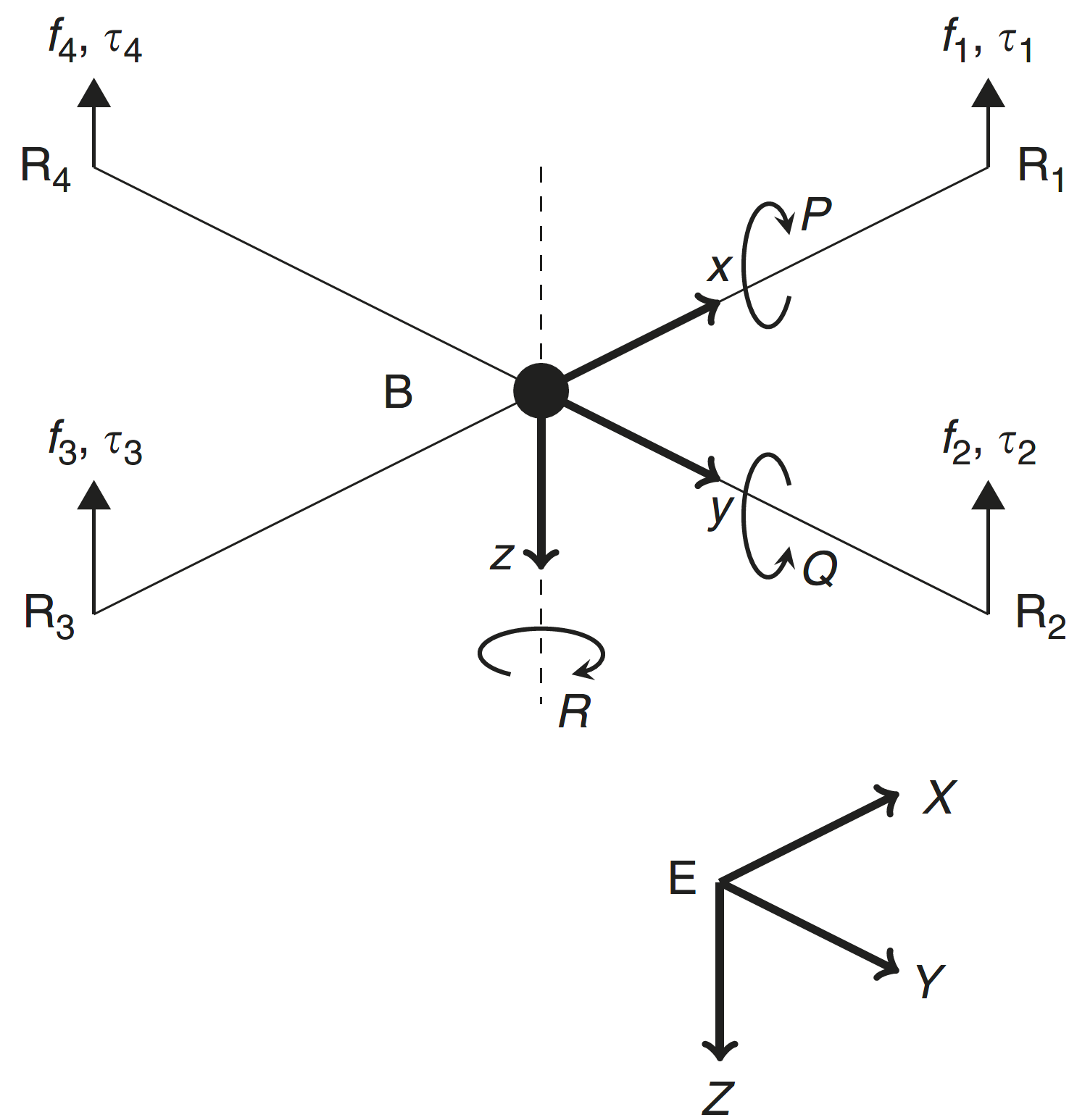
The basic vehicle configuration, Earth frame, E, and body frame, B, are shown in Figure 1 The body frame has the axes originating at the center of mass of the vehicle. An inertial coordinate frame is fixed to the Earth and has axes in the conventional North-East-Down arrangement. It is assumed that the Earth is flat and stationary. Each rotor provides a thrust force, f_i, and torque, τ_i. These combine to a vector of moments about the body axis, M = [L,M,N] and a thrust force in the negative z-direction, −T. The orthogonal rotation matrix S_b to transform from body frame to Earth frame is

```latex\mathbf{S}_{b}=\begin{bmatrix}c_{\theta}c_{\psi}&c_{\theta}s_{\psi}&-s_{\theta}\\s_{\phi}s_{\theta}c_{\psi}-c_{\phi}s_{\psi}&c_{\phi}c_{\psi}+s_{\phi}s_{\theta}s_{\psi}&c_{\theta}s_{\phi}\\c_{\phi}s_{\theta}c_{\psi}+s_{\phi}s_{\psi}&c_{\phi}s_{\theta}s_{\psi}-s_{\phi}c_{\psi}&c_{\theta}c_{\phi}\end{bmatrix},```

(1)

where c_θ denotes cos⁡θ,s_θ denotes sin⁡θ, etc., and (ϕ,θ,ψ) is the standard Euler angle roll-pitch-yaw triplet. The gravitational force vector, F_g, in the body axis is

```latex\mathbf{F}_g=m\mathbf{S}_b\begin{bmatrix}0\\0\\g\end{bmatrix}=mg\begin{bmatrix}-s_\theta\\c_\theta s_\phi\\c_\theta c_\phi\end{bmatrix},```

(2)

where g is gravitational field constant which is taken as g = 9.81 N kg⁻¹. The Newton-Euler equations of motion of the body axes frame are

```latex\begin{array}{rl}\mathbf{F}&=m\dot{\mathbf{V}}+\omega\times m\mathbf{V},\\\mathbf{M}&=\mathbf{I}\dot{\omega}+\omega\times\mathbf{I}\omega\end{array}```

(3)

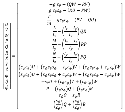
where V = [U,V,W]^T is the vector of velocities in the body frame, ω = [P,Q,R]^T is the vector of angular rates in the body frame, I = diag⁡(I_x,I_y,I_z) is the moments of inertia matrix, m is the mass of the vehicle, F = F_g + [0,0,–T]^T is the vector of the forces acting on the center of mass, and M = [L,M,N]^T is the vector of moments acting about the center of mass. A general state space model is obtained from [35] with state variables given by

```latex\mathbf{x}=[U\,V\,W\,P\,Q\,R\,X\,Y\,Z\,\phi\,\theta\,\psi]^{T}.```

(4)

The resulting model is

(5)

The moments acting on the quadrotor L, M and N and the total force T are given by

```latex\begin{bmatrix}T\\L\\M\\N\end{bmatrix}=\begin{bmatrix}1&1&1&1\\0&-\ell&0&\ell\\\ell&0&-\ell&0\\-d&d&-d&d\end{bmatrix}\begin{bmatrix}T_1\\T_2\\T_3\\T_4\end{bmatrix}```

(6)

with l is the arm length d is the rotor diameter. The general state space formulation can be written as follows

```latex\dot{\mathbf{x}}=f(\mathbf{x},\mathbf{U}),```

(7)

with

```latex\mathbf{U}=[\begin{matrix}T_1&&T_2&&T_3&&T_4\end{matrix}]^T.```

The objective is to compute the control input vector U(t) to force the system outputs to track their desired trajectories using ℒ₁ adaptive control.

Figure 1. Quadrotor Frames.

2.2. ℒ₁ Adaptive Control Design A common procedure in adaptive control design is to linearize the nonlinear model at a given equilibrium or operating point, in order to develop a linear controller based on the linearized system model, and to augment the linear controller with the adaptive controller. This allows for better robustness of the system. Actually, it permits for a less “burden” of the adaptive controller through the use of the prior knowledge of the system [40]. Linearizing about the hover equilibrium state, x_eq and control, u_eq gives

```latex\delta\dot{\mathbf{x}}=\mathbf{A}\delta\mathbf{x}+\mathbf{B}\delta\mathbf{u}```

(8)

where δx and δu represents the small perturbations of the state and control about x_eq and u_eq respectively, where

```latex\mathbf{A}=\begin{bmatrix}0_{1\times6}&0_{1\times3}&0_{1\times1}&-g&0_{1\times1}\\0_{1\times6}&0_{1\times3}&g&0_{1\times1}&0_{1\times1}\\0_{4\times6}&0_{4\times3}&0_{4\times1}&0_{4\times1}&0_{4\times1}\\\mathbb{I}_{6}&0_{6\times3}&0_{6\times1}&0_{6\times1}&0_{6\times1}\end{bmatrix}```

and

```latex\mathbf{B}=\begin{bmatrix}0_{5\times1}&0_{5\times3}\\-\frac{1}{m}&0_{1\times3}\\0_{3\times1}&0_{3\times3}\\0_{3\times1}&\mathbf{I}^{-1}\end{bmatrix}\begin{bmatrix}1&1&1&1\\0&-\ell&0&\ell\\\ell&0&-\ell&0\\-d&d&-d&d\end{bmatrix}.```

Consequently, the non-linear model of the quadrotor in Equation (7) can be formulated as the following class of MIMO uncertain systems

```latex\begin{aligned}&\dot{\mathbf{x}}(t) =\mathbf{A}_{p}\mathbf{x}(t)+\mathbf{B}_{p}\mathbf{u}_{p}(t)+\mathbf{h}(t,\mathbf{x}),\mathbf{x}(0)=\mathbf{x}_{0}, \\&\mathbf{y}(t) =\mathbf{Cx}(t), \end{aligned}```

(9)

where $$\mathbf{A}_p=\mathbf{A}+\Delta\mathbf{A}\in\mathbb{R}^{n\times n} $$ is an unknown matrix, $$\mathbf{A}\in\mathbb{R}^{n\times n}$$ is a known matrix, Δ$$\mathbf{A}\in\mathbb{R}^{n\times n}$$ an unknown matrix of the system dynamics, $$\mathbf{B}_{p}=\mathbf{B}(\mathbb{I}_{m}+\Delta\mathbf{B})\in\mathbb{R}^{n\times m}$$ is an unknown matrix, $$\mathbf{B}\in\mathbb{R}^{n\times m}$$ is a known matrix, Δ$$\mathbf{B}\in\mathbb{R}^{n\times m}$$ is an unknown matrix of the control input uncertainties, $$\mathbf{C}\in\mathbb{R}^{m\times n}$$ is a known matrix, $$\mathbf{x}(t)\in\mathbb{R}^n$$ is the state vector which is assumed to be available through measurement, $$\mathbf{u}_p(t)\in\mathbb{R}^m$$ is the control input vector and $$\mathbf{h}(t,x)\in\mathbb{R}^{n}$$ is a vector of unknown nonlinear functions. This formulation is a general case of MIMO systems, and it is quite understood that for a quadrotor n = 12 and m = 4. Now consider the control law

```latex\mathbf{u}_p(t)=\mathbf{u}(t)+\mathbf{K}_l\mathbf{x}(t),```

(10)

where $$\mathbf{K}_{l}\in\mathbb{R}^{m\times n}$$ is a gain matrix that defines A_m = A + BK_l, where $$\mathbf{A}_{m}\in\mathbb{R}^{n\times n}$$ is a Hurwitz matrix that defines the desired dynamics of the system. The resulting system to be controlled by the adaptive control is:

```latex\dot{\mathbf{x}}(t)=\mathbf{A}_{m}\mathbf{x}(t)+\mathbf{B}\omega\mathbf{u}(t)+\tilde{\mathbf{h}}(t,\mathbf{x}),```

(11)

where $$\omega=\mathbb{I}_{m}+\Delta\mathbf{B}\mathrm{\,and\,}\tilde{\mathbf{h}}(t,\mathbf{x})=\Delta\mathbf{A}\mathbf{x}(t)+(\omega-\mathbb{I}_{m})\mathbf{K}_{l}\mathbf{x}(t)+\mathbf{h}(t,\mathbf{x})$$. For control design, $$\tilde{\mathbf{h}}(t,\mathbf{x})$$ can be modelled as follows

```latex\tilde{\mathbf{h}}(t,\mathbf{x})=\mathbf{B}\big(\boldsymbol{\theta}\mathbf{x}(t)+\sigma_{m}(t)\big)+\mathbf{B}_{u}\sigma_{u}(t).```

(12)

Hence, the system in (11) can be parametrized as follows

```latex\dot{\mathbf{x}}(t)=\mathbf{A}_{m}\mathbf{x}(t)+\mathbf{B}\big(\omega\mathbf{u}(t)+\boldsymbol{\theta}\mathbf{x}(t)+\boldsymbol{\theta}_{m}(t)\big)+\mathbf{B}_{u}\sigma_{u}(t),```

(13)

where $$\theta\in\mathbb{R}^{m\times n}$$ is a matrix of constant unknown parameters representing model uncertainties, $$\sigma_m(t)\in\mathbb{R}^m$$ is an unknown matched disturbance, $$\sigma_u(t)\in\mathbb{R}^n$$ is an unknown unmatched disturbance, and $$\mathbf{B}_{u}\in\mathbb{R}^{n\times(n-m)}$$ is a constant matrix such that $$\mathbf{B}^{T}\mathbf{B}_{u}=0$$ and $$[\mathbf{BB}_{um}]$$ has rank n. Assumption 1. The unknown model parameters are bounded, i.e., $$\boldsymbol{\theta}\in\Theta$$, where Θ is a known compact convex set. The system input gain matrix ω is assumed to be an unknown (non-singular) strictly row-diagonally dominant matrix with sgn⁡(ω_ii ) known. Furthermore, it is assumed that there exists a known compact convex set Ω such that $$\omega\in\Omega\subset\mathbb{R}^{m\times m}$$. The disturbances σ_m(t) and σ_u(t) are bounded, i.e., σ_m ∈ Δ_m and σ_u ∈ Δ_u, where Δ_m and Δ_u are known compact sets. Finally σ_m(t) and σ_u(t) are assumed to be differentiable with bounded derivatives, i.e. there exist finite real $$d_{\sigma_m}$$ and $$d_{\sigma_u}$$ such that

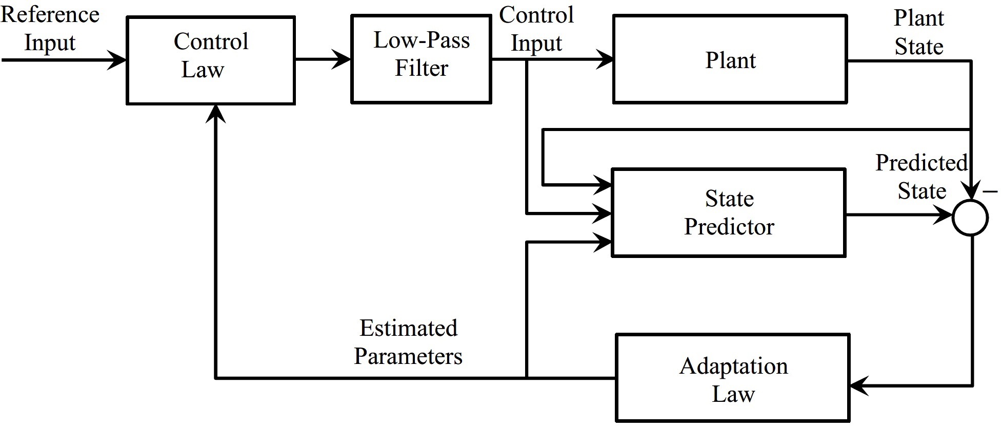
```latex\left\|\dot{\boldsymbol{\sigma}}_{m}(t)\right\|_{2}\leq\boldsymbol{\sigma}_{m},\left\|\dot{\boldsymbol{\sigma}}_{u}(t)\right\|_{2}\leq\boldsymbol{\sigma}_{u}\forall t\geq0.```

We consider the architecture of the ℒ₁ adaptive controller [26] which is composed of the state predictor, the adaptation law and the control law (Figure 2).

Figure 2. Block diagram of the ℒ<sub>1</sub> adaptive controller.

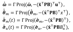
The state predictor is defined by

```latex\dot{\hat{\mathbf{x}}}(t)=\mathbf{A}_{m}\hat{\mathbf{x}}(t)+\mathbf{B}\left(\hat{\omega}(t)\mathbf{u}(t)+\hat{\boldsymbol{\theta}}(t)\mathbf{x}(t)+\hat{\boldsymbol{\sigma}}_{m}(t)\right)+\mathbf{B}_{u}\hat{\boldsymbol{\sigma}}_{\mathbf{u}}(t),```

(14)

where $$\hat{\boldsymbol{\omega}}(t),\hat{\boldsymbol{\theta}}_m(t),\hat{\boldsymbol{\sigma}}_m(t)$$, and $$\hat{\boldsymbol{\sigma}}_u(t)$$ are the estimates of the unknown system parameters and $$\mathbf{\hat{x}}(t)$$ is the estimate of the state vector x(t). The adaptation laws are given by

(15)

where $$\mathbf{\tilde{x}}=\mathbf{\hat{x}}-\mathbf{x}$$ is the prediction errors, Γ > 0 are the adaptation gains, and P is the solution of the algebraic Lyapunov equation $$\mathbf{A}_{m}^{\top}\mathbf{P}+\mathbf{P}\mathbf{A}_{m}=-\mathbf{Q},\mathbf{Q}>0$$, while Proj⁡(⋅,⋅) denotes the projection operator defined over the sets Θ,Ω,Δ_m and Δ_u. To define the control law, we need to introduce some notations. Let

```latex\begin{bmatrix}\mathbf{H}_{xm}(s)\\\mathbf{H}_{xum}(s)\end{bmatrix}=(s\mathbb{I}-\mathbf{A}_m)^{-1}\begin{bmatrix}\mathbf{B}_m\\\mathbf{B}_u\end{bmatrix}\\\begin{bmatrix}\mathbf{H}_m(s)\\\mathbf{H}_{um}(s)\end{bmatrix}=\mathbf{C}\begin{bmatrix}\mathbf{H}_{xm}(s)\\\mathbf{H}_{xum}(s)\end{bmatrix}```

The control law is given by

```latex\mathbf{u}(s)=\mathbf{KF}(s)\Big(\mathbf{K}_{g}\mathbf{r}(s)-\hat{\boldsymbol{v}}(s)\Big),```

(16)

where $$\hat{\boldsymbol{v}}(s)=\hat{\boldsymbol{v}}_1(s)+\hat{\boldsymbol{v}}_2(s),\hat{\boldsymbol{v}}_1(s)$$ is the Laplace transformation of $$\hat{\boldsymbol{v}}_{1}(t)=\hat{\boldsymbol{\omega}}(t)\mathbf{u}(t)+\hat{\boldsymbol{\sigma}}_{m}(t),\hat{\boldsymbol{v}}_{2}(s)=H_{m}^{-1}(s)H_{um}(s)\hat{\boldsymbol{\sigma}}_{u}(s)$$, $$\mathbf{K}_{g}=-(\mathbf{CA}_{m}^{-1}\mathbf{B})^{-1}$$ is the pre-filter of the MIMO control law, F(s) is a m × m strictly proper transfer function matrix and $$\mathbf{K}\in\mathbb{R}^{m\times m}$$. For analysis purposes, without loss of generality, F(s) is chosen as $$\mathbf{F}(s)=\frac{\mathbf{D}(s)}{s}$$, where D(s) is a proper stable transfer function. Hence, the control law can be written:

```latex\mathbf{u}(s)=K\frac{\mathbf{D}(s)}{s}\Big(\mathbf{K}_{g}r(s)-\hat{v}(s)\Big),```

(17)

which leads, for all ω ∈ Ω, to a strictly proper stable

```latex\mathbf{G}(s)\triangleq\omega\mathbf{KD}(s)\big(s\mathbb{I}_{m}+\omega\mathbf{KD}(s)\big)^{-1},```

with DC gain $$\mathbf{G}(0)=\mathbb{I}_m$$. The ℒ₁ adaptive controller is subject to the ℒ₁ norm condition [26]

```latex\begin{aligned}L&=\max_{\boldsymbol{\theta}\in\Theta}\parallel\boldsymbol{\theta}\parallel_{\mathcal{L}_{1}}=\max_{i}\bigl(\sum\nolimits_{j}\bigl|\boldsymbol{\theta}_{ij}\bigr|\bigr),\\\overline{\mathbf{G}}(s)&=(s\mathbb{I}-vA_{m})^{-1}\mathbf{B}\big(\mathbb{I}-\mathbf{G}(s)\big).\end{aligned}```

(18)

where ∥⋅∥_ℒ₁. denotes for the ℒ₁ norm. Moreover, the choice of D(s) also needs to ensure that $$\mathbf{C}(s)\mathbf{H}_{m}^{-1}(s)$$ is a proper stable transfer matrix. In the next section is presented the analysis of hard failures effect on quadrotor dynamics that leads to the inversion of the torque.

3. Quadrotor Hard Failures Analysis

If a fault or failure occurs on the system, the unknown parameters may go outside the predefined sets. As a consequence, the stability condition [26] may become not satisfied. More particularly, in case of a structural, hardware or software failure, the direction of the force vector of a propeller might be inverted. This is a very critical situation for pitch and roll angles, because the torques N and M will act in the opposite direction to the desired commands N_c and M_c, and the system will become unstable. 3.1. Case Study: Quadrotor Modeling in Case of Structural Damage or Payload Shift Quadrotor UAVs are increasingly being used for package delivery. Because the content or the package itself might shift during the flight, centre of gravity (COG) variation occurs. As the centre of gravity affects the flight dynamics of the quadrotor, the performance of the UAV is degraded, if the centre of gravity does not coincide with the geometric centre of the quadrotor. The shift of the centre of gravity might occur also in case of structural damage. It is straightforward to show that in the case of shift of the centre the expression of the forces and moments acting on the UAV formulated in (6) will be reformulated as follows

```latex\begin{bmatrix}T\\L\\M\\N\end{bmatrix}=\begin{bmatrix}1&1&1&1\\0&-\ell+\delta_y&0&\ell+\delta_y\\\ell-\delta_x&0&-\ell-\delta_x&0\\-d&d&-d&d\end{bmatrix}\begin{bmatrix}T_1\\T_2\\T_3\\T_4\end{bmatrix},```

(19)

where δ_x and δ_y are the distances of shift of the COG that are assumed to be unknown. It is clear that the sign of the diagonal of the control input depends on the amplitude of the shift of the centre of gravity and on the sign of −l − δ_x and −l + δ_x, consequently. If the centre of gravity shift goes beyond limits, the sign of the diagonals of the input matrix B can be reverted and leads to the instability of the control system. 3.2. Case Study: Rotor Aerodynamic Modelling in Case of Blades Damage The thrust T produced by the rotation of the blades can be expressed [41,42] by

```latex\mathrm{T}=C_T\rho A(\zeta R)^2,```

(20)

where ρ is the density of air, A is the area captured by rotor, R is the rotor radius, ζ is the angular speed of the rotor and C_T the thrust coefficient. When a rotorcraft rolls and pitches, the rotors experience a vertical velocity, leading to a change in the inflow angle. In this case the thrust coefficient C_T can be related to the vertical velocity V_c as [43]

```latex\frac{C_{\mathrm{T}}}{\sigma}=\frac{a(\alpha)}{4}\biggl[\theta_{\mathrm{tip}}-\frac{v_{i}+V_{c}}{\zeta R}\biggr],```

(21)

where a is the airfoil polar lift slope, θ_tip is the geometric blade angle at the tip of the rotor, v_i is the induced velocity through the rotor, and σ is the solidity of the disc-the ratio of the surface area of the blades and the rotor disc area. The added lift due to increased flow velocity magnitude at the blade is small relative to the effect of changing inflow angle, and is ignored [43]. It is possible that blade damage or icing can induce a change in the sign of the thrust coefficient. This could be a consequence of:

A reduction of the geometric blade angle θ_tip.
An augmentation of the induced velocity v_i and/or the vertical velocity V_c.
A change of the direction of the polar lift slope a(α), that is a highly nonlinear for some airfoils [43].

Remark 1. Based on the previous analysis, it is necessary to maintain system stability and a minimum of good performance, this is done through the design of a set of degraded models which become effective when large uncertainties appear on the plant.

4. Multiple Model ℒ₁ Adaptive Control of MIMO Systems

In this section, the multiple model ℒ₁ adaptive controller first presented in [39] is extended to MIMO systems. Considering probable faults scenario, a set of plant parameterizations, based on multiple models, is arranged, and the objective is that the satisfactory controller is selected automatically to deal with every situation. This means that the model which is the best match of the plant is selected. The desired performance of each model is made through the design of the pair $$(\mathbf{A}_{m(i)},\mathbf{B}_i)$$, for i = 0…M_d, where M_d is the number of degraded models. The system in (9) can consequently be parameterized as follows

```latex\begin{aligned}&\dot{\mathbf{x}}(t) =\mathbf{A}_{m(i)}\mathbf{x}(t)+\mathbf{B}_{i}\left(\omega_{i}\mathbf{u}(t)+\boldsymbol{\theta}_{i}\mathbf{x}(t)+\sigma_{m(i)}(t)\right)+\mathbf{B}_{u(i)}\sigma_{u(i)}(t), \\&\mathbf{y}(t) =\mathbf{Cx}(t), \end{aligned}```

(22)

where $$\mathbf{A}_{m(i)}\in\mathbb{R}^{n\times n}$$ are known Hurwitz matrices that define the desired dynamics of the system $$\mathbf{B}_{i}\in\mathbb{R}^{n\times m}$$ are the desired input matrices, $$\omega_{i}\in\mathbb{R}^{m\times m}$$ are unknown constant matrices representing the system input gain, $$\mathbf{B}_{u(i)}\in\mathbb{R}^{n\times n-m}$$ are the unmatched disturbances matrices, $$\boldsymbol{\theta}_{i}\in\mathbb{R}^{m\times n}$$ are matrices of unknown parameters, $$\boldsymbol{\sigma}_{m(i)}(t)\in\mathbb{R}^{m}$$ are unknown matched disturbances, σ_u(i)(t) ∈ $$\mathbb{R}^{n-m}$$ are unknown unmatched disturbances. $$\mathbf{C}\in\mathbb{R}^{m\times n}$$ is the output matrix and $$\mathbf{y}(t)\in\mathbb{R}^{m}$$ is the output vector. Assumption 2. The system input gain matrices ω_i are assumed to be unknown (non-singular) strictly row-diagonally dominant matrices with known signs of diagonals. 4.1. 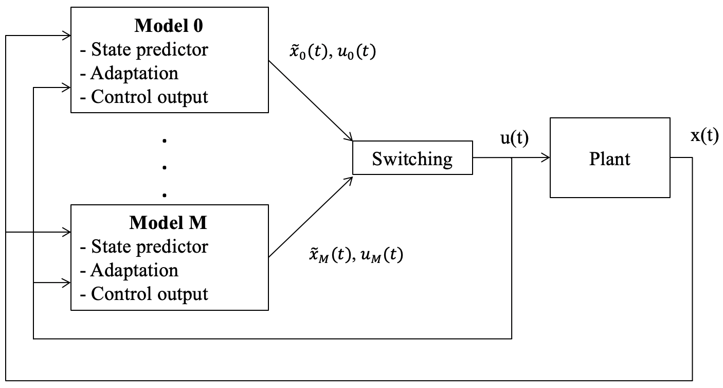Controller Design The multiple model ℒ₁ adaptive controller, as shown in Figure 3, is composed of a set of state predictors, a set of adaptation laws, a set of control laws and a control input selector (switching system). 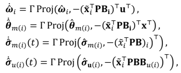The state predictors are defined by

```latex\dot{\hat{\mathbf{x}}}_i(t)=\mathbf{A}_{m(i)}\hat{\mathbf{x}}_i(t)+\mathbf{B}_i\left(\hat{\boldsymbol{\omega}}_i(t)\mathbf{u}(t)+\hat{\boldsymbol{\theta}}_i\mathbf{x}(t)+\hat{\boldsymbol{\sigma}}_{m(i)}(t)\right)+\mathbf{B}_{u(i)}\hat{\boldsymbol{\sigma}}_{u(i)}(t),```

(23)

where $$\mathbf{\hat{x}}_{i}(t)$$ are the predicted states and, $$\hat{\boldsymbol{\theta}}_i(t),\hat{\boldsymbol{\omega}}_i(t),\hat{\boldsymbol{\theta}}_{m(i)}(t),\hat{\boldsymbol{\sigma}}_{m(i)}(t)$$, and $$\hat{\boldsymbol{\sigma}}_{\mathcal{U}(i)}(t)$$ are the estimates of the unknown system parameters and external disturbances. The initial state of the state predictor is equal to the plant state at switching time t_k :

```latex\hat{\mathbf{x}}(t_{k})=\mathbf{x}(t_{k}).```

The adaptation laws are given by

(24)

where $$\mathbf{\tilde{x}}_{i}=\mathbf{\hat{x}}_{i}-\mathbf{x}$$ are the prediction errors, Γ_i > 0 are the adaptation gains and P is the solution of the algebraic Lyapunov equation $$\mathbf{A}_{m(i)}^{\top}\mathbf{P}+\mathbf{P}\mathbf{A}_{m(i)}=-\mathbf{Q},\mathbf{Q}>0$$. To define the control law, let:

```latex\begin{bmatrix}\mathbf{H}_{xm(i)}(s)\\\mathbf{H}_{xum(i)}(s)\end{bmatrix}=\begin{pmatrix}s\mathbb{I}-\mathbf{A}_{m(i)}\end{pmatrix}^{-1}\begin{bmatrix}\mathbf{B}_{(i)}\\\mathbf{B}_{u(i)}\end{bmatrix}\\\begin{bmatrix}\mathbf{H}_{m(i)}(s)\\\mathbf{H}_{um(i)}(s)\end{bmatrix}=\mathbf{C}\begin{bmatrix}\mathbf{H}_{xm(i)}(s)\\\mathbf{H}_{xum(i)}(s)\end{bmatrix}```

The control laws are given by

```latex\mathbf{u}_{i}(s)=\mathbf{K}_{i}\mathbf{F}_{i}(s)\Big(\mathbf{K}_{g(i)}\mathbf{r}(s)-\hat{v}_{i}(s)\Big),```

(25)

where $$\hat{v}_{i}(s)=\hat{v}_{1(i)}(s)+\hat{v}_{2(i)}(s),\hat{v}_{1(i)}(s)$$ are the Laplace transformations of $$\hat{v}_{1(i)}(t)=\hat{\omega}(t)\mathbf{u}(t)+\hat{\boldsymbol{\sigma}}_{m(i)}(t),\hat{v}_{2(i)}(s)=$$ $$\mathbf{H}_{m(i)}^{-1}(s)\mathbf{H}_{um(i)}(s)\hat{\boldsymbol{\sigma}}_{u(i)}(s),\mathbf{K}_{g(i)}=-\big(\mathbf{CA}_{m(i)}^{-1}\mathbf{B}_{i}\big)^{-1}$$ are the pre-filters of the MIMO control laws, F_i(s) are m × m strictly proper transfer function matrices and $$\mathbf{K}\in\mathbb{R}^{m\times m}$$. Similarly to ℒ₁ adaptive control with one model, F_i(s) are chosen as $$\mathbf{F}_{i}(s)=\frac{\mathbf{D}_{i}(s)}{s}$$, where D_i(s) are proper stable transfer functions. Hence, the control laws can be written as

```latex\mathbf{u}_{i}(s)=\mathbf{K}_{i}\frac{\mathbf{D}_{i}(s)}{s}\Big(\mathbf{K}_{g(i)}r(s)-\hat{v}_{i}(s)\Big),```

(26)

which leads, for all ω ∈ Ω, to a strictly proper stable

```latex\mathbf{G}_{i}(s)\triangleq\omega_{i}\mathbf{K}_{i}\mathbf{D}_{i}(s)\big(s\mathbb{I}_{m}+\boldsymbol{\omega}_{i}\mathbf{K}_{i}\mathbf{D}_{i}(s)\big)^{-1},```

with DC gain $$G_{i}(0)=\mathbb{I}_{m}$$. The switching logic is defined by

```latex\min_{i=0..M_{d}}\Big\{J_{i}=c_{1}\|\tilde{\mathbf{x}}_{i}\|^{2}+c_{2}\int_{0}^{t}e^{-c_{3}(t-\tau)}\|\tilde{\mathbf{x}}_{i}(\tau)\|^{2}d\tau\Big\},```

(27)

where c₁,c₂ and c₃ are arbitrary positive reals. The model that minimizes the criterion becomes the selected model.

Figure 3. Block diagram of the multiple model ℒ<sub>1</sub> adaptive controller.

4.2. Controller Analysis In this section, the performance of the ℒ₁ adaptive controller is analysed. More specifically it is shown that:

The reference models resulting from perfect knowledge of the uncertainties and a corresponding non-adaptive controller are stable, subject to some conditions involving the filters F_i(s).
The prediction errors, i.e., the errors between the states of the plant and those of the state predictors, are bounded.
The differences between the states/input of the system and those of the reference systems are proportional to the prediction error

4.2.1. Reference Models Analysis For a switching system, it is not straightforward to compute the ℒ₁ norm condition in Equation (18). Actually, for LTI systems, the ℒ₁ norm is readily computed from the impulse response. However, for a switched system, the impulse response is time dependent (switching signal-dependent), and computing the ℒ₁ norm is not as straightforward as in the LTI case. In consequence, the approach proposed in [44] is extended here to the case of systems with unmatched disturbances. For each parametrization, the reference model with the nominal parameters of the system is defined by

```latex\dot{\mathbf{x}}_{r}(t)=\mathbf{A}_{(i)}\mathbf{x}_{r}(t)+B_{i}\left(\omega_{i}\mathbf{u}_{r}(t)+\sigma_{m(i)}(t)\right)+\sigma_{u(i)}(t).```

(28)

The reference (nominal) control law is given by

```latex\mathbf{u}_{r(i)}(s)=K_{i}\frac{D_{i}(s)}{s}\Big(\mathbf{K}_{g(i)}\mathbf{r}_{i}(s)-\boldsymbol{v}_{(i)}(s)\Big),```

(29)

where $$\boldsymbol{v}_{(i)}(s)=\boldsymbol{v}_{1(i)}(s)+\boldsymbol{v}_{2(i)}(s)\boldsymbol{\sigma}_{u(i)}(s),\boldsymbol{v}_{1(i)}(s)$$ are the Laplace transformations of $$\boldsymbol{v}_{1(i)}(s)=\omega_{i}(t)\mathbf{u}_{i}(t)+\boldsymbol{\sigma}_{m(i)}(t)$$, v₂ = $$\mathbf{H}_{m(i)}^{-1}(s)\mathbf{H}_{0(i)}(s)\boldsymbol{\sigma}_{u(i)}(s),\mathbf{K}_{g(i)}=-\left(\mathbf{C}_i\mathbf{A}_{(i)}^{-1}\mathbf{B}_i\right)^{-1}$$ are the pre-filters of the MIMO control laws, D_i(s) are m × m strictly proper transfer matrices and $$\mathbf{K}_{i}\in\mathbb{R}^{m\times m}$$. 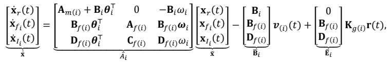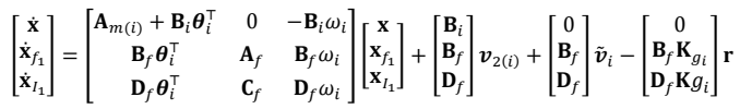Letting $$(\mathbf{A}_{f(i)},\mathbf{B}_{f(i)},\mathbf{C}_{f(i)},\mathbf{D}_{f(i)})$$ be a minimal realization of D_i(s) with n_f(i) states, the reference system dynamics can be written in state-space form as follows

(30)

where $$\mathbf{x}_{f_{i}},\mathbf{x}_{l_{i}}$$ are the states of the filters and the integrators, respectively, and $$\mathbf{\bar{x}}(0)=[\mathbf{x}_{0}^{\mathsf{T}},0,0]^{\mathsf{T}}$$. The reference control law can be written as follows

```latex\mathbf{u}_{r(i)}(t)=\underbrace{\begin{bmatrix}0&0&-\mathbb{I}\end{bmatrix}}_{\bar{c}}\begin{bmatrix}\mathbf{x}_r(t)\\\mathbf{x}_{f_i}(t)\\\mathbf{x}_{l_i}(t)\end{bmatrix}.```

(31)

The system in (30) and (31) is equivalent to:

```latex\begin{aligned}&\dot{\bar{\mathbf{x}}}=\overline{\mathbf{A}}_{i}\bar{\mathbf{x}}+\overline{\mathbf{B}}_{i}\boldsymbol{v}_{(i)}+\bar{\mathbf{E}}_{i}\mathbf{K}_{g(i)}\mathbf{r}(t),\\&\mathbf{u}_{r(i)}=\bar{\mathbf{C}}\bar{\mathbf{x}}.\end{aligned}```

(32)

Remark 2. In this work it is assumed that the switching is arbitrary, i.e., not dwell time or average dwell time. The switching signal has a dwell time τ > 0, if the switching times satisfy $$t_{k+1}-t_{k}\geq\tau,\forall k>0$$ [45]. Lemma 1. Give an arbitrary matrix $$\mathbf{Q}=\mathbf{Q}^{\mathsf{T}}>0$$, if there exists a constant symmetric matrix P > 0 verifying

```latex\overline{\mathbf{A}}_i^\top\mathbf{P}+\mathbf{P}\overline{\mathbf{A}}_i\leq-\mathbf{Q},\forall\boldsymbol{\theta}_i\in\Theta_i\mathrm{~and~}\forall\omega_i\in\Omega_i,```

then the Lyapunov function $$V={\bar{\mathbf{x}}}^{\top}{\bar{\mathbf{P}}}{\bar{\mathbf{x}}}$$ guarantees the stability of the switching reference systems in (30) and (31). This fact is straightforward from the converse Lyapunov theorem for LTI systems. 4.2.2. Transient Performance and Steady-State Performance In the following Lemma, it is stated that the prediction errors $$\mathbf{\tilde{x}}_{i}(t)$$ and the estimation errors of the unknown parameters are bounded for i = 0…M_d. 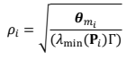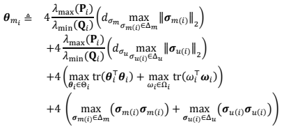Lemma 2. The prediction error of each state predictor, $$\mathbf{\tilde{x}}_{i}(t)$$ is bounded with respect to initial conditions and its bound is given by

```latex\|\tilde{\mathbf{x}}_{i}\|_{\mathcal{L}_{\infty}}\leq\rho_{i},```

(33)

where

and

Proof Let $$\tilde{\boldsymbol{\theta}}_{i}=\hat{\boldsymbol{\theta}}_{i}-\boldsymbol{\theta}_{i},\tilde{\boldsymbol{\sigma}}_{m(i)}=\hat{\boldsymbol{\sigma}}_{m(i)}-\sigma_{m(i)},\tilde{\boldsymbol{\sigma}}_{u(i)}=\hat{\boldsymbol{\sigma}}_{u(i)}-\sigma_{u(i)},\tilde{\boldsymbol{\omega}}_{i}=\hat{\boldsymbol{\omega}}_{i}-\omega_{i}$$, the following error dynamics can be derived from (13) and (22)

```latex\tilde{\mathbf{x}}_{i}=\mathbf{A}_{m(i)}\tilde{\mathbf{x}}_{i}+\mathbf{B}_{i}\big(\tilde{\boldsymbol{\omega}}_{i}\mathbf{u}+\tilde{\boldsymbol{\theta}}_{i}\mathbf{x}+\tilde{\boldsymbol{\sigma}}_{m(i)}\big)+\tilde{\boldsymbol{\sigma}}_{u(i)},```

(34)

with $$\mathbf{\tilde{x}}_{i}(0)$$ = 0 Consider the following Lyapunov functions

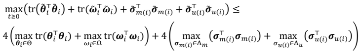
```latexV_i=\tilde{\mathbf{x}}_i^\top\mathbf{P}_i\tilde{\mathbf{x}}_i+\Gamma^{-1}\operatorname{tr}(\tilde{\boldsymbol{\theta}}^{i\top}\tilde{\boldsymbol{\theta}}_i)+\Gamma^{-1}\operatorname{tr}(\tilde{\boldsymbol{\omega}}^{i\top}\tilde{\boldsymbol{\omega}}_i)\\+\Gamma^{-1}\big(\tilde{\boldsymbol{\sigma}}_{m(i)}^\top\tilde{\boldsymbol{\sigma}}_{m(i)}\big)+\Gamma^{-1}\big(\tilde{\boldsymbol{\sigma}}_{u(i)}^\top\tilde{\boldsymbol{\sigma}}_{u(i)}\big)```

(35)

Using the adaptation laws from (24), the derivatives of the Lyapunov functions are bounded as follows

(36)

The projection algorithm ensures that $$\hat{\boldsymbol{\theta}}_{i}\in\Theta,\hat{\Omega}_{i}\in\omega,\hat{\sigma}_{m(i)}\in\Delta_{m}\mathrm{~and~}\hat{\sigma}_{u(i)}\in\Delta_{u}$$. Consequently, it can be written

(37)

If $$V_i\geq\boldsymbol{\theta}_{m(i)}\Gamma $$ at some time t, then it follows that

(38)

Using the bounds in assumption 1, it can be written

(39)

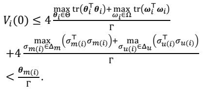
Consequently, if $$V_{i}\geq\frac{\theta_{m(i)}}{\Gamma_{i}}$$, then it follows that

```latex\dot{V}_{i}\leq0.```

(40)

Given that $$\tilde{\mathbf{x}}_{i}(0)=0$$, we have

(41)

Recalling that

```latex\lambda_{\min}(\mathbf{P}_i)\|\tilde{\mathbf{x}}_i\|^2\leq\tilde{\mathbf{x}}_\mathbf{i}^\top\mathbf{P}_i\bar{\mathbf{x}}_i\leq V_i,```

(42)

which implies that

```latex\left\|\bar{\mathbf{x}}_{i}\right\|_{2}^{2}\leq\frac{\theta_{m(i)}}{\lambda_{\min}(\mathbf{P}_{i})\Gamma},```

(43)

and consequently

```latex\left\|\bar{\mathbf{x}}_i\right\|_2\leq\rho_i.```

(44)

The proof is complete. The following theorem shows that the states of the adaptive system follow those of the reference system with a bound proportional to $$\parallel\tilde{\mathbf{x}}\parallel_{\mathcal{L}_{\infty}}$$. The approach is similar to [44], for the case of arbitrary switching. Theorem. If the reference system is exponentially stable then

```latex\left\|\mathbf{x}_{r}-\mathbf{x}\right\|_{\mathcal{L}_{\infty}}\leq\kappa_{2}\parallel\tilde{\mathbf{x}}\parallel_{\mathcal{L}_{\infty}},\left\|\mathbf{u}_{r}-\mathbf{u}\right\|_{\mathcal{L}_{\infty}}\leq\kappa_{3}\parallel\tilde{\mathbf{x}}\parallel_{\mathcal{L}_{\infty}}```

where κ₂ and κ₃ are positive constants defined in (57) and (60), respectively. Proof. The control laws in (26) can be written as

```latex\mathbf{u}(s)=-\frac{D_{0}(s)}{s}\big(\omega_{i}\mathbf{u}(s)+v_{i}(s)+\tilde{v}_{i}(s)-\mathbf{K}g_{i}\mathbf{r}(s)\big),```

(45)

where $$\tilde{\boldsymbol{v}}_{(i)}(s)=\tilde{\boldsymbol{v}}_{1(i)}(s)+\tilde{\boldsymbol{v}}_{2(i)}(s),\tilde{\boldsymbol{v}}_{1(i)}(s)$$ are the Laplace transformations of $$\tilde{\boldsymbol{v}}_{1(i)}=\tilde{\boldsymbol{\theta}}_{i}^{\top}\mathbf{x}(t)+\tilde{\boldsymbol{\omega}}_{i}(t)\mathbf{u}(t)\mathrm{\,and\,}\tilde{\boldsymbol{v}}_{2(i)}(s)=$$ $$\tilde{\boldsymbol{\sigma}}_{\mathbf{u}(i)}(s)+\mathbf{H}_{m(i)}^{-1}(s)\mathbf{H}_{0(i)}(s)\tilde{\boldsymbol{\sigma}}_{u(i)}(s)$$. Consequently, the closed-loop systems (22) and (45) can be written as follows

(46)

The error between the state of the reference system and the actual plant, e = x_r − x, can be expressed as

(47)

The control error can also be formulated as follows

```latex\mathbf{e}_u=\mathbf{u}_r-\mathbf{u}=\begin{bmatrix}0&0&-\mathbb{I}\end{bmatrix}\begin{bmatrix}\mathbf{e}\\\mathbf{x}_{f_1}\\\mathbf{x}_{I_1}\end{bmatrix}```

(48)

The prediction error dynamics in (34) can be written as

```latex\tilde{\mathbf{v}}_{i}=\mathbf{B}_{i}^{\dagger}\big(\dot{\tilde{\mathbf{x}}}-\mathbf{A}_{m(i)}\tilde{\mathbf{x}}\big).```

(49)

Passing $$\mathbf{B}_{i}^{\dagger}\dot{\tilde{\mathbf{x}}}$$ through the filter $$(s\mathbb{I}+D_{0}(s)\omega_{i})^{-1}D_{0}(s)$$, we can write

```latex\begin{bmatrix}\dot{\mathbf{x}}_{f_2}\\\dot{\mathbf{x}}_{I_2}\end{bmatrix}=\begin{bmatrix}\mathbf{A}_f&\mathbf{B}_f\omega_i\\\mathbf{C}_f&\mathbf{D}_f\omega_i\end{bmatrix}\begin{bmatrix}\mathbf{x}_{f_2}\\\mathbf{x}_{I_2}\end{bmatrix}+\begin{bmatrix}\mathbf{B}_f\\\mathbf{D}_f\end{bmatrix}\mathbf{B}_i^\dagger\tilde{\mathbf{x}}```

(50)

Applying this to the error dynamics in (47) we have

```latex\begin{bmatrix}\dot{\mathbf{e}}\\\dot{\mathbf{x}}_{f_1}\\\dot{\mathbf{x}}_{f_1}\\\dot{\mathbf{x}}_{f_2}\\\dot{\mathbf{x}}_{t_2}\end{bmatrix}=\begin{bmatrix}\mathbf{A}_{m(i)}+\mathbf{B}_{i}\boldsymbol{\theta}_{i}^{\top}&0&-\mathbf{B}_{i}\omega_{i}&-\mathbf{B}_{i}\mathbf{C}_{f}&-\mathbf{B}_{i}\mathbf{D}_{f}\omega_{i}\\\mathbf{B}_{f}\boldsymbol{\theta}_{i}^{\top}&\mathbf{A}_{f}&\mathbf{B}_{f}\omega_{i}&0&0\\\mathbf{D}_{f}\boldsymbol{\theta}_{i}^{\top}&\mathbf{C}_{f}&\mathbf{D}_{f}\omega_{i}&0&0\\0&0&0&\mathbf{A}_{f}&\mathbf{B}_{f}\omega_{i}\\0&0&0&\mathbf{C}_{f}&\mathbf{D}_{f}\boldsymbol{\omega}_{i}\end{bmatrix}\begin{bmatrix}\mathbf{e}\\\mathbf{x}_{f_1}\\\mathbf{x}_{f_2}\\\mathbf{x}_{f_2}\\\mathbf{x}_{t_2}\end{bmatrix}+\begin{bmatrix}-\mathbf{D}_{f}\mathbf{B}_{i}^{\dagger}\\-\mathbf{B}_{f}\mathbf{B}_{i}^{\dagger}\mathbf{A}_{m(i)}\\-\mathbf{D}_{f}\mathbf{B}_{i}^{\dagger}\mathbf{A}_{m(i)}\\-\mathbf{B}_{f}\mathbf{B}_{i}^{\dagger}\\-\mathbf{D}_{f}\mathbf{B}_{i}^{\dagger}\end{bmatrix}\tilde{\mathbf{x}},```

(51)

and

```latex\mathbf{e}_{u}=[0\quad0\quad-\mathbb{I}\quad-\mathbf{C}_{f}\quad-\mathbf{D}_{f}\omega_{i}]\begin{bmatrix}\mathbf{e}\\\mathbf{x}_{f1}\\\mathbf{x}_{l_{1}}\\\mathbf{x}_{l_{2}}\\\mathbf{x}_{l_{2}}\end{bmatrix}+[-\mathbf{D}_{f}\mathbf{B}_{i}^{\dagger}]\tilde{\mathbf{x}}.```

(52)

Letting

```latex\begin{aligned}&\bar{\mathbf{H}}_{i}=\begin{bmatrix}-\mathbf{B}_{i}\mathbf{C}_{f}&-\mathbf{B}_{i}\mathbf{D}_{f}\omega_{i}\\0&0\\0&0\end{bmatrix},\bar{\mathbf{J}}_{i}=\begin{bmatrix}-\mathbf{D}_{f}\mathbf{B}_{i}^{\dagger}\\-\mathbf{B}_{f}\mathbf{B}_{i}^{\dagger}\mathbf{A}_{m(i)}\\-\mathbf{D}_{f}\mathbf{B}_{i}^{\dagger}\mathbf{A}_{m(i)}\end{bmatrix},\\&\bar{\mathbf{G}}_{i}=\begin{bmatrix}-\mathbf{B}_{f}\mathbf{B}_{i}^{\dagger}\mathbf{A}_{(i)}\\-\mathbf{D}_{f}\mathbf{B}_{i}^{\dagger}\mathbf{A}_{(i)}\end{bmatrix},\bar{\mathbf{L}}_{i}=[0\quad\mathbf{C}_{f}\quad\mathbf{D}_{f}\omega_{i}],\end{aligned}```

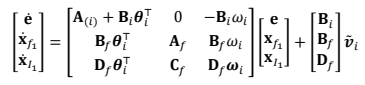
it follows from (51) and (52) that

```latex\begin{bmatrix}\dot{\bar{\mathbf{e}}}\\\dot{\mathbf{x}}_{f_2}\end{bmatrix}=\begin{bmatrix}\overline{\mathbf{A}}_i&\overline{\mathbf{H}}_i\\0&\overline{\mathbf{F}}_i\end{bmatrix}\begin{bmatrix}\bar{\mathbf{e}}\\\bar{\mathbf{x}}_{f_2}\end{bmatrix}+\begin{bmatrix}\bar{\mathbf{J}}_i\\\bar{\mathbf{G}}_i\end{bmatrix}\tilde{\mathbf{x}},```

(53)

and

```latex\mathbf{e}_{u}=[\bar{\mathbf{C}}\quad\bar{\mathbf{L}}_{i}]\begin{bmatrix}\bar{\mathbf{e}}\\\bar{\mathbf{x}}_{f_{2}}\end{bmatrix}+[-\mathbf{D}_{f}\mathbf{B}_{i}^{\dagger}]\tilde{\mathbf{x}},```

(54)

where $$\bar{\mathbf{e}}=\left[\mathbf{e}^{\mathsf{T}},\mathbf{x}_{f_{1}}^{\mathsf{T}},\mathbf{x}_{l_{1}}^{\mathsf{T}}\right]^{\mathsf{T}}$$ and $${\bar{\mathbf{x}}}_{f_{2}}=\left[\mathbf{x}_{f_{2}}^{\mathsf{T}},\mathbf{x}_{l_{2}}^{\mathsf{T}}\right]^{\mathsf{T}}$$. Note that the reference system is stable and the filter represented by $$\bar{\mathbf{F}}_{i}$$ is a subsystem of the reference system when θ = 0. Therefore, from Lemma 1, there exists positive definite matrices $$\mathbf{Q}_{i}(\omega_{i})>0$$ such that for all ω_i ∈ Ω,

```latex\mathbf{\bar{F}}_{i}^{\top}\mathbf{\bar{Q}}_{i}+\mathbf{\bar{Q}}_{i}\mathbf{\bar{F}}_{i}\leq-\mathbb{I}.```

(55)

Let $$\bar{V}_{i}(t)=\bar{\mathbf{x}}_{f_{2}}^{\top}\bar{\mathbf{Q}}_{i}\bar{\mathbf{x}}_{f_{2}}$$, where V_i(0) =0. Differentiating along the system trajectories it follows that

```latex\begin{aligned}\dot{V}_{i}& =\bar{\mathbf{x}}_{f_{2}}^{\top}(\bar{\mathbf{F}}_{i}^{\top}\bar{\mathbf{Q}}_{i}+\bar{\mathbf{Q}}_{i}\bar{\mathbf{F}}_{i})\bar{\mathbf{x}}_{f_{2}}+2\bar{\mathbf{x}}_{f_{2}}^{\top}\bar{\mathbf{Q}}_{i}\bar{\mathbf{G}}_{i}\tilde{\mathbf{x}} \\&\leq-\|\bar{\mathbf{x}}_{f_{2}}\|^{2}+2\|\bar{\mathbf{x}}_{f_{2}}\|\beta_{F}\parallel\tilde{\mathbf{x}}\parallel_{\mathcal{L}_{\infty}} \\&\leq-\|\bar{\mathbf{x}}_{f_{2}}\|^{2}+\beta_{F}^{2}\parallel\tilde{\mathbf{x}}\parallel_{\mathcal{L}_{\infty}}^{2}\end{aligned}```

(56)

where the last line follows from square completion and $$\beta_{F}=\sqrt{n}\mathrm{max}_{i\in I}\|\bar{\mathbf{Q}}_{i}\bar{\mathbf{G}}_{i}\|$$. By integrating it is straightforward to show that the following bound holds for $$\mathbf{\bar{x}}_{f_{2}}$$

```latex\|\bar{\mathbf{x}}_{f_{2}}\|_{\mathcal{L}_{\infty}}\leq\kappa_{1},```

(57)

where $$\kappa_{1}=\sqrt{n}\mathrm{max}_{i\in I}\|\overline{\mathbf{Q}}_{i}\overline{\mathbf{G}}_{i}\|\delta $$ and δ is the upper bound of $$\tilde{\mathbf{x}}_i $$ defined in Lemma 2. We now define the Lyapunov functions $$\bar{W}_{i}=\bar{\mathbf{e}}^{\top}\bar{\mathbf{P}}_{i}\bar{\mathbf{e}}$$. Differentiating along the system trajectories it follows that

```latex\begin{aligned}\dot{W}_{i}& =\bar{\mathbf{e}}^\top(\overline{\mathbf{A}}_i^\top\overline{\mathbf{P}}_i+\overline{\mathbf{P}}_i\overline{\mathbf{A}}_i)\bar{\mathbf{e}}+2\bar{\mathbf{e}}^\top\overline{\mathbf{P}}_i\overline{\mathbf{H}}_i\bar{\mathbf{x}}_{f_2}+2\bar{\mathbf{e}}^\top\overline{\mathbf{P}}_i\bar{\mathbf{J}}_i\tilde{\mathbf{x}} \\&\leq-\parallel\bar{\mathbf{e}}\parallel^2+2\parallel\bar{\mathbf{e}}\parallel\beta_{\bar{e}}\parallel\tilde{\mathbf{x}}\parallel_{\mathcal{L}_{\infty}} \\&\leq-\parallel\bar{\mathbf{e}}\parallel^2+\beta_{\bar{e}}^2\parallel\tilde{\mathbf{x}}\parallel_{\mathcal{L}_\infty}^2,\end{aligned}```

(58)

where $$\beta_{e}=\begin{pmatrix}\kappa_{1}\max_{i\in I}\|\overline{\mathbf{P}}_{i}\overline{\mathbf{H}}_{i}\|+\sqrt{n}\max_{i\in I}\|\overline{\mathbf{P}}_{i}\overline{\mathbf{J}}_{i}\|\end{pmatrix}$$. Therefore, the following bound holds

```latex\parallel\bar{\mathbf{e}}\parallel_{L_{\infty}}\leq\kappa_{2},```

(59)

where $$\kappa_{2}=\bigl(\kappa_{1}\mathrm{max}_{i\in I}\|\overline{\mathbf{P}}_{i}\overline{\mathbf{H}}_{i}\|+\sqrt{n}\mathrm{max}_{i\in I}\|\overline{\mathbf{P}}_{i}\overline{\mathbf{J}}_{i}\|\bigr)\delta $$. Given the definition of e_u from (54), it follows that

```latex\begin{aligned}\left\|\mathbf{e}_{u}\right\|_{\mathcal{L}_{\infty}}\leq&\leq\parallel\bar{\mathbf{C}}\parallel\parallel\bar{\mathbf{e}}\parallel_{\mathcal{L}_{\infty}}+\parallel\bar{\mathbf{L}}_{i}\parallel\parallel\bar{\mathbf{x}}_{f_{2}}\parallel_{\mathcal{L}_{\infty}}+\parallel\mathbf{D}_{f}\mathbf{B}_{i}^{\dagger}\parallel\parallel\tilde{\mathbf{x}}\parallel_{\mathcal{L}_{\infty}},\\&\leq\kappa_{3},\end{aligned}```

(60)

where $$\kappa_3=\parallel\bar{\mathbf{C}}\parallel\kappa_2+(\mathrm{max}_{i\in I}\|\bar{\mathbf{L}}_i\|+\mathrm{max}_{i\in I}\|\mathbf{D}_f\mathbf{B}_i^\dagger\|)\delta $$. This completes the proof.

5. Simulation Results for Quadrotor Control in Case of Inversion of the Torque Direction

In this section, the simulation results for the ℒ₁ adaptive controller with a single model and multiple models are presented and compared. The vehicle that is modelled for use in this work is the Draganfly X-pro quadrotor. The quadrotor arm length is 0.50 m. Each rotor has two blades. The radius of the rotor is 0.258 m, and the mean chord of the blade is 0.032 m. A 14.8 V lithium-ion polymer battery is used for supplying the electric power, this being the maximum voltage that can be supplied to a motor [35]. The mass and inertia parameters are [46,47]:

```latexm=2.356\,\mathrm{kg},I_{x}=0.1676\,\mathrm{kg}\,\mathrm{m}^{2}\\I_{y}=0.1676\,\mathrm{kg\,m}^{2},I_{z}=0.29743\,\mathrm{kg\,m}^{2}```

The rotors are driven by voltages to four electronic motors, the thrust-voltage relationship can be expressed as follows

```latexf_i=k_fv_i^2,i=1,2,3,4```

where f_i is the individual thrust from i th rotor, v_i is the individual voltage input and $$k_{f}=\frac{0.11\mathrm{N}}{\mathrm{V}^{2}}$$. The individual torque of each rotor is

```latex\tau_i=k_\tau v_i^2```

where τ_i is the individual torque from i th rotor and $$k_{\tau}=\frac{0.052\mathrm{Nm}}{\mathrm{V}^{2}}$$. The force and moments are not linear with voltage, but linear with squared voltage, therefore the squared voltages are used as the final full system model input vector, $$u=[v_{1}^{2},v_{2}^{2},v_{3}^{2},v_{4}^{2}]^{T}$$. The system of Equation (9) with its nominal desired dynamics can be parameterized to become similar to the class of MIMO systems in (22) defined by

```latex\dot{\mathbf{x}}(t)=\mathbf{A}_{(0)}\mathbf{x}(t)+B_{0}\left(\omega_{0}u(t)+\theta_{0}^{\mathsf{T}}\mathbf{x}(t)+\sigma_{m(0)}(t)\right)+\mathbf{B}_{u}\sigma_{u(0)}```

The bounds for the unknown time-varying parameters for the implementation of the projection operator were ω₀ ∈ [0.25,1.25], $$\theta_{0}\in[-25,25],\sigma_{m(0)}\in[-30,30]\mathrm{~and~}\sigma_{u(0)}\in[-30,30]$$. The adaptation gain is Γ = 1000. The filter parameters were

```latexK_0=\begin{bmatrix}160&0&0&0\\0&160&0&0\\0&0&160&0\\0&0&0&160\end{bmatrix}D_0(s)=\frac{1}{s}\begin{bmatrix}1&0&0&0\\0&1&0&0\\0&0&1&0\\0&0&0&1\end{bmatrix}.```

It is straightforward to verify that the design verifies the stability condition in (18). The performance of the ℒ₁ adaptive controller has been compared with the indirect Multiple Model Reference Adaptive Controller (M-MRAC) presented in [48]. Our aim is not to compare the two designs, as it has already been shown in [49] that the tracking performance and disturbance rejection of the MRAC controller are better with increasing adaptation gain. However, the MRAC controller exhibits poor attenuation of high-frequency content in the presence of large adaptation gain. On the other hand, the ℒ₁ adaptive controller shows good disturbance rejection within the controller bandwidth in the presence of fast adaptation. However, the performance of the ℒ₁ adaptive controller is limited by the low-pass filter. Simulations were first made using only the nominal controller, i.e., the ℒ₁ adaptive and the MRAC controllers with only the nominal model. The adaptation gain of the MRAC is Γ = 50. The objective is to change the altitude of the quadrotor while maintain it at the same horizontal (x,y) position. Two situations were considered in this case:

Loss of effectiveness in rotor 1 of 50%;
Loss of effectiveness in rotor 1 of 50% with the inversion of the thrust direction.

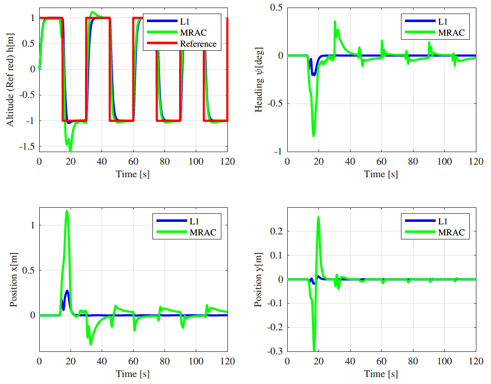
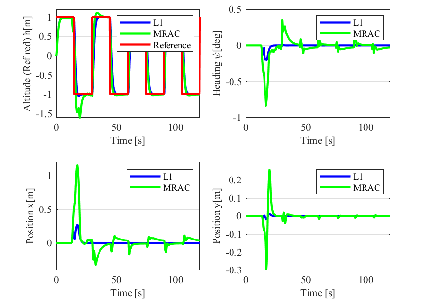
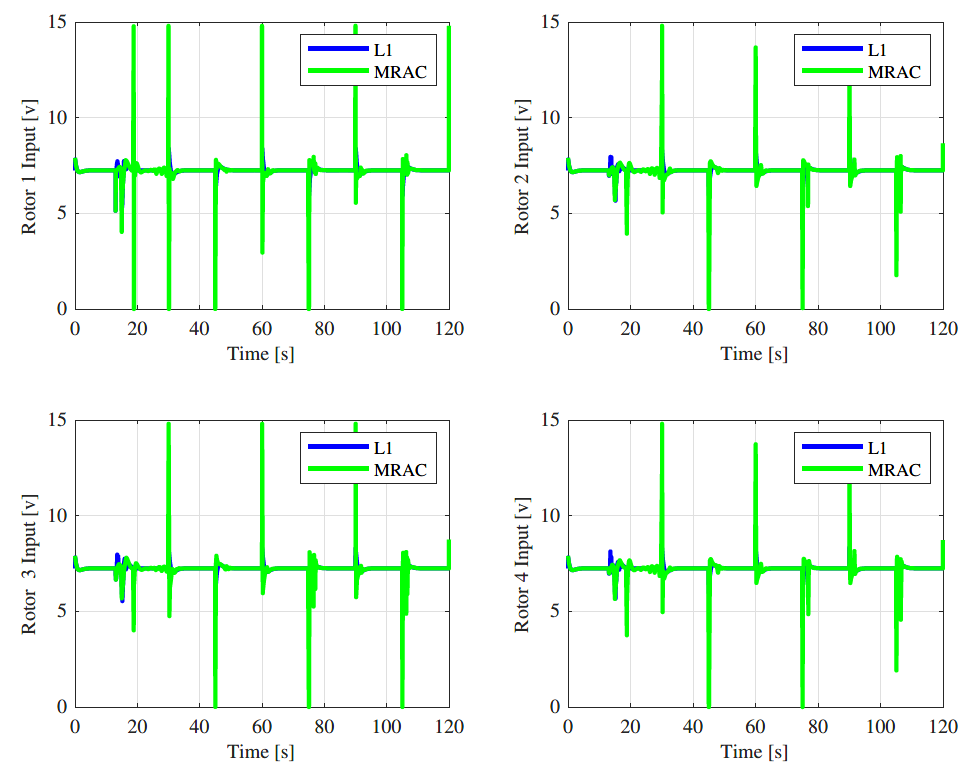
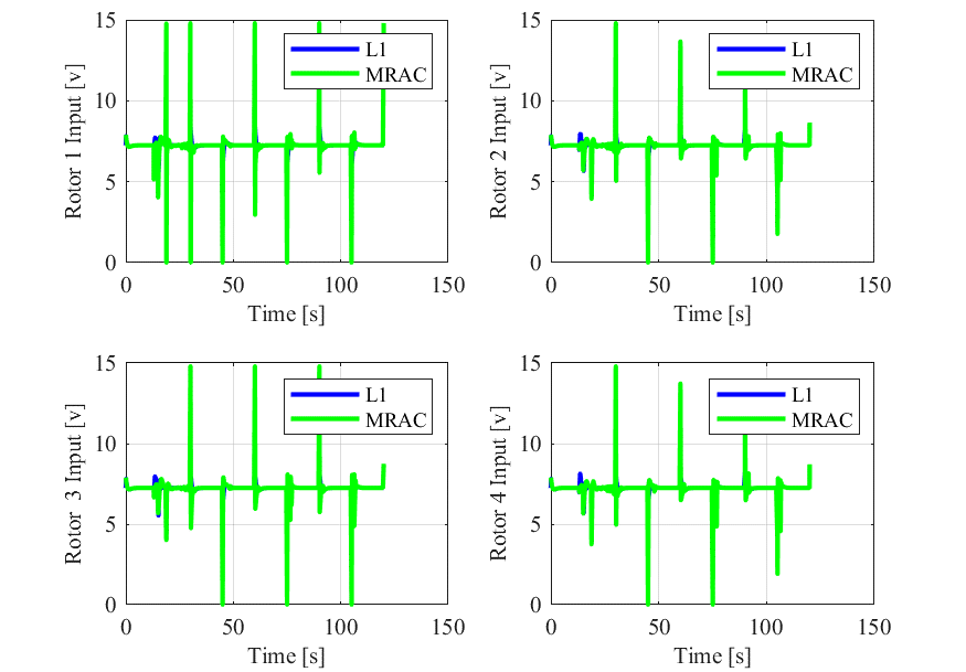
The failures were introduced at simulation time t = 13 s. Simulation results for the nominal ℒ₁ adaptive controller and the MRAC, without inversion of rotor signs, are shown in Figure 4. As expected, the system has good performance subsequent to the fault. The loss of altitude is within acceptable limits. Displacements in the X and Y positions are not meaningful. As expected, the ℒ₁ adaptive controller shows better performance in transient regime, following the occurrence of the failure, while the MRAC is better in permanent regime. The rotor commands are within acceptable limits as it can be observed in Figure 5. 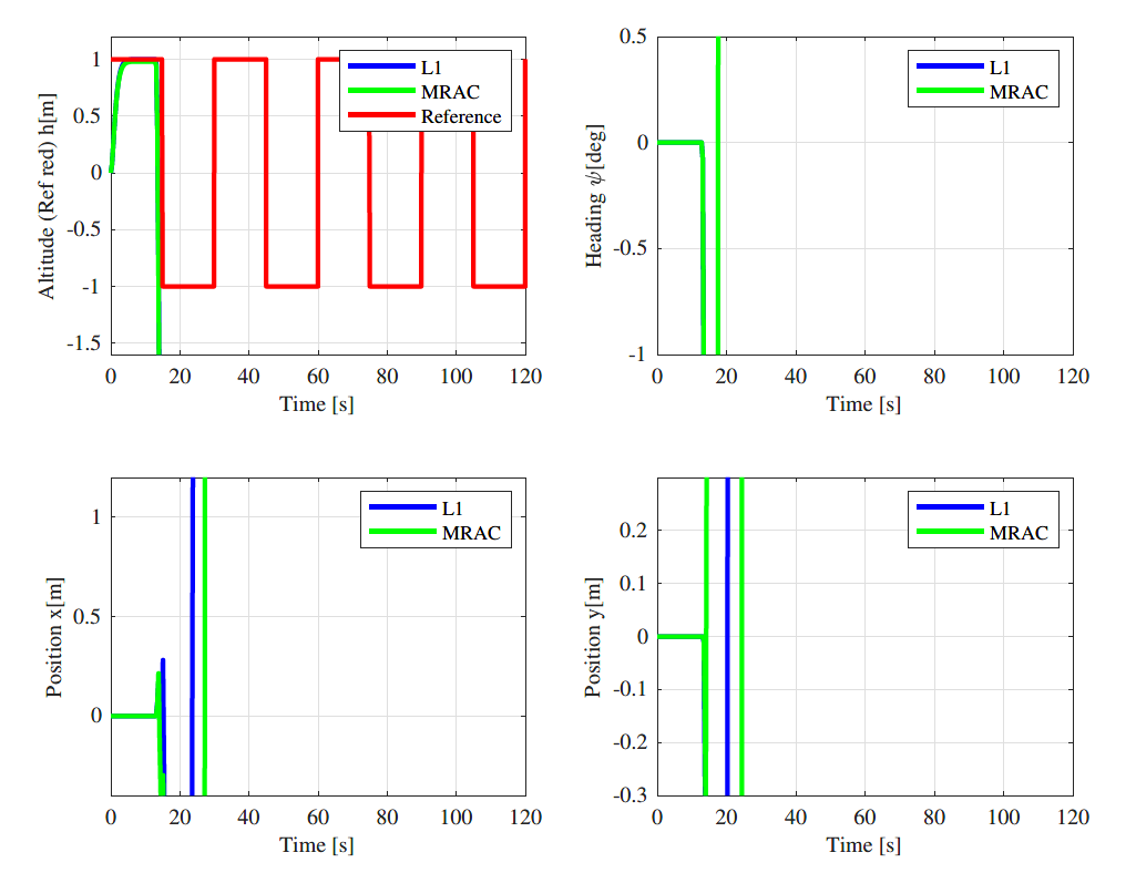In the second scenario of loss of effectiveness of 50% with the inversion of the sign of the thrust, the system with only the nominal controller has become unstable for both ℒ₁ adaptive controller and MRAC, as it can be observed in Figure 6. Next, the multiple model controller was applied. It was based on the nominal controller and four degraded controllers designed to deal with possible inversion of rotor commands.

Figure 4. Closed-loop tracking performance of the nominal controller without inversion of the sign of the thrust.

Figure 5. Control input to the rotors without inversion of the sign of the thrust.

Figure 6. Closed-loop tracking performance of the nominal controller with inversion of the sign of the thrust.

A second model for the case of inversion of the sign of rotor 1 command is given by

```latex\dot{\mathbf{x}}(t)=\mathbf{A}_{(1)}\mathbf{x}(t)+\mathbf{B}_{0}\beta_{1}\big(\omega_{1}u(t)+\boldsymbol{\theta}_{1}^{\intercal}\mathbf{x}(t)+\sigma_{m(1)}\big)+\mathbf{B}_{u}\sigma_{u(1)}```

where β₁ = diag⁡(−1,1,1,1). A third model for the case of inversion of the sign of rotor 2 command is given by

```latex\dot{\mathbf{x}}(t)=\mathbf{A}_{(2)}\mathbf{x}(t)+\mathbf{B}_{0}\beta_{2}\big(\omega_{2}\mathbf{u}(t)+\mathbf{\theta}_{2}^{\intercal}\mathbf{x}(t)\sigma_{m(2)}\big)+\mathbf{B}_{u}\sigma_{u(2)},```

where β₂ = diag⁡(1,−1,1,1). A fourth model for the case of inversion of both the signs of rotor 3 command is given by

```latex\dot{\mathbf{x}}(t)=\mathbf{A}_{(3)}\mathbf{x}(t)+\mathbf{B}_{0}\beta_{3}\big(\omega_{3}\mathbf{u}(t)+\boldsymbol{\theta}_{3}^{\intercal}\mathbf{x}(t)+\sigma_{m(3)}\big)+\mathbf{B}_{u}\sigma_{u(3)},```

where β₃ = diag⁡(1,1,−1,1). A fifth model for the case of inversion of both the signs of rotor 3 command is given by

```latex\dot{\mathbf{x}}(t)=\mathbf{A}_{(3)}\mathbf{x}(t)+\mathbf{B}_{0}\beta_{4}\big(\omega_{3}u(t)+\boldsymbol{\theta}_{3}^{\intercal}\mathbf{x}(t)+\sigma_{m(4)}\big)+\mathbf{B}_{u}\sigma_{u(4)},```

where β₄ = diag⁡(1,1,1,−1). The input matrix B₀ was taken to be the same for all models. The adaptation gain of the M-MRAC is Γ = 50. The filter parameters of the ℒ₁ adaptive controller were the same as for the single model controller. Comparing with (30), the minimum realisation of D_i is

```latex\mathbf{A}_f=0,\mathbf{B}_f=0,\mathbf{C}_f=\begin{bmatrix}1&0&0&0\\0&1&0&0\\0&0&1&0\\0&0&0&1\end{bmatrix},\mathbf{D}_f=0.```

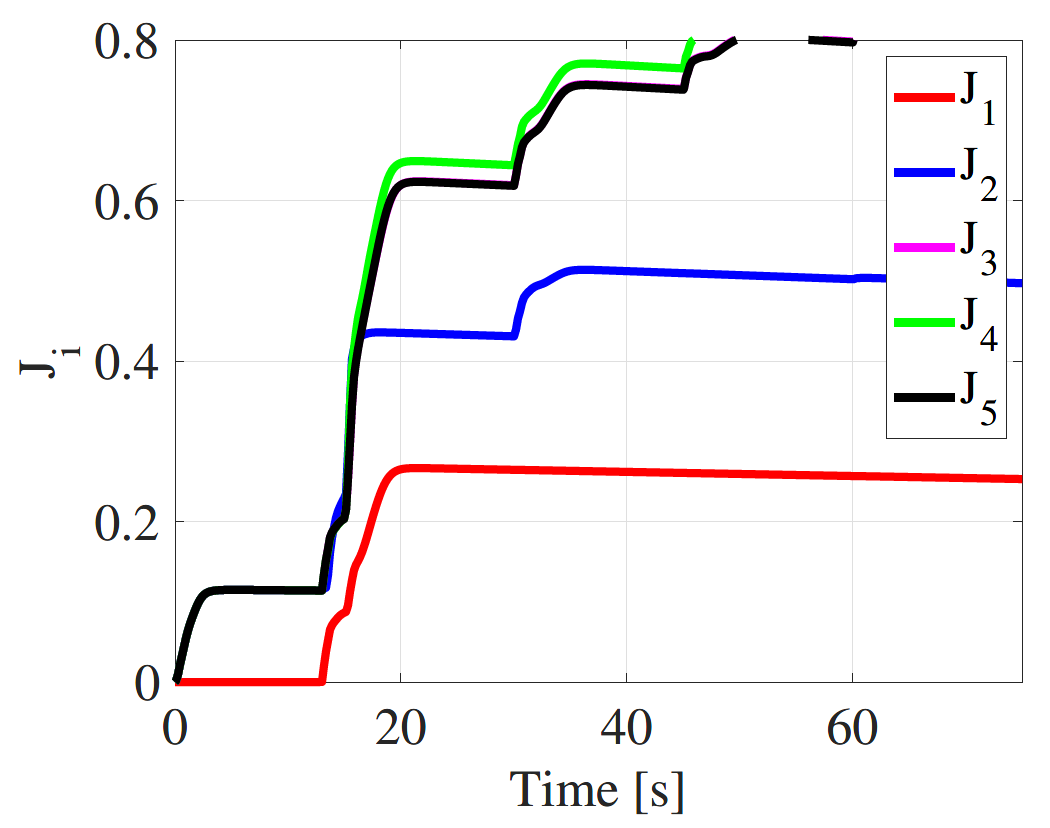
The tuning parameters and the desired dynamics of the degraded controller were the same as the nominal controller. By defining the system similarly to (30), the stability condition of the reference system in Lemma 2 was verified using a common Lyapunov function. The previous failure cases were reproduced for the multiple model controller. The simulation results in the case of non inversion of the sign of propeller 1 are shown in Figure 7 and Figure 8. The system has same behaviour than a single model controller. Furthermore, as it is shown on Figure 9, the matching model is the nominal model which corresponds on the minimum cost function defined in (27).

Figure 7. Closed-loop tracking performance of the multiple model controller without inversion of the sign of the thrust.

Figure 8. Control input of the quadrotor using the multiple model controller without inversion of the sign of the thrust.

Figure 9. Switching Function without of inversion of the sign of the thrust.

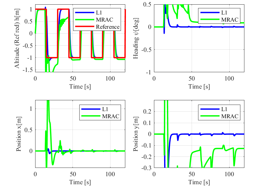
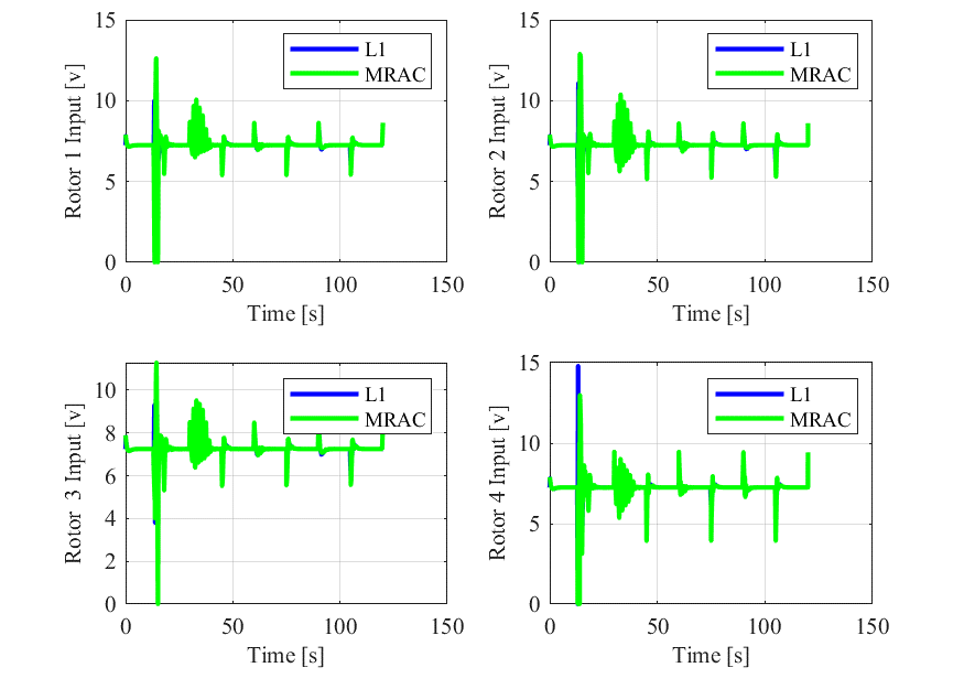
For the second case of the inversion it can be seen in Figure 10 and Figure 11 that the system has remained stable and shows good tracking performance. The aileron voltage commands to the propellers are within acceptable limits. It is worth noting that, in this case, the M-MRAC is exhibiting relatively poor performance when compared to the ℒ₁ adaptive controller. This is attributed to the slow transient regime, and the attempt to enhance performance by increasing adaptation gains resulted in worse performance, as high-frequency oscillations in the control input were observed. 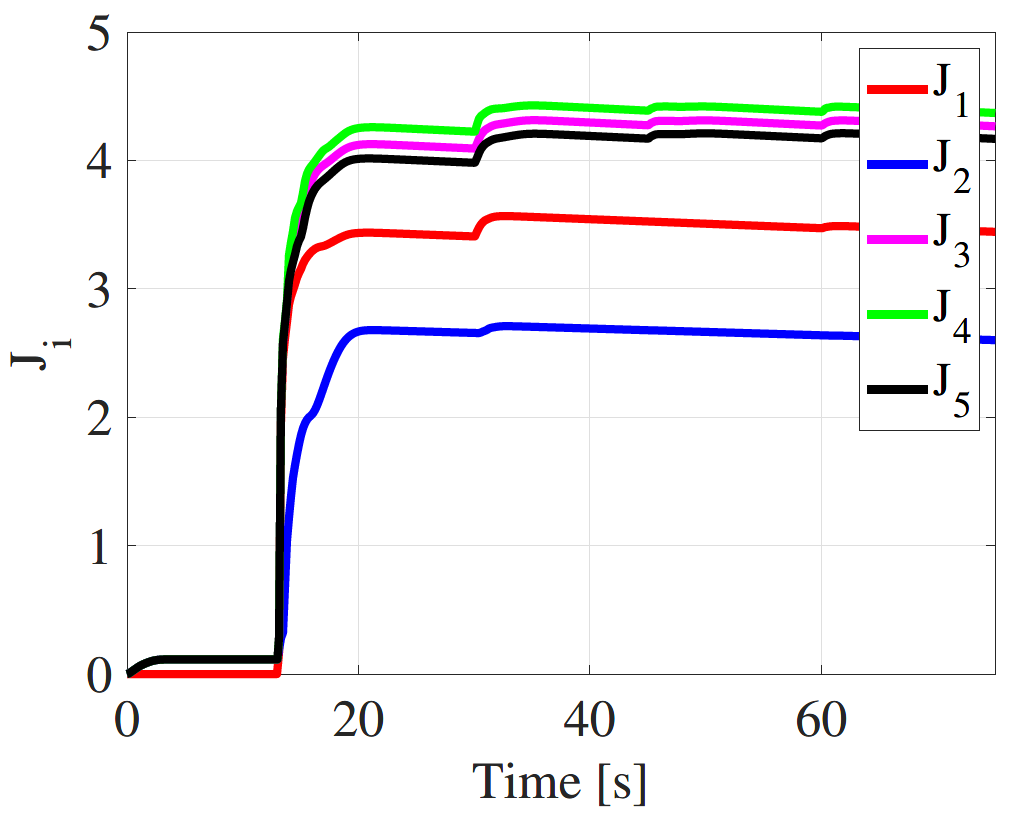Furthermore, it is shown in Figure 12, the matching model is model 1, which corresponds to the minimum cost function defined in (27). These simulations demonstrate that the application of the multiple model ℒ₁ adaptive controller is justified in case of structural damages or faults that lead to inversion of the sign of the control input of quadrotor UAVs.

Figure 10. Closed-loop tracking performance of the multiple model controller in case of inversion of the sign of the thrust.

Figure 11. Control input of the multiple model controller in case of inversion of the sign of the thrust.

Figure 12. Switching Function in case of inversion of the sign of the thrust.

6. Summary

In this paper, an approach for fault-tolerant control of quadrotor UAVs in the presence of critical failure was presented based on ℒ₁ adaptive control. The design is based on a nominal model for the plant in the presence of soft faults and a set of degraded models for the plant under critical failures. The switching between the models is based on a simple quadratic criterion. The main advantage of this approach is that it allows a larger class of uncertainties and faults to be considered and can achieve better fault accommodation and preserve system integrity. Simulations have shown that the multiple model ℒ₁ adaptive has stabilized the system in case of inversion of the control input, while the controller with a single model failed.

Nomenclature

Author Contributions

All authors have contributed equally to the paper.

Funding

This research received no external funding.

Declaration of Competing Interest

Data Availability Statement

The data that support the findings of this study are available from the corresponding author toufik.souanef@cranfield.ac.uk, upon reasonable request.

References

Bouabdallah S, Noth A, Siegwart R. PID vs LQ control techniques applied to an indoor micro quadrotor. In Proceedings of the 2004 IEEE/RSJ International Conference on Intelligent Robots and Systems (IROS), 28 September–02 October 2004, Sendai, Japan; Volume 3, pp. 2451–2456.

Tayebi A, McGilvray S. Attitude stabilization of a VTOL quadrotor aircraft. IEEE Trans. Control Syst. Technol. 2006, 14, 562–571. [Google Scholar]

Marks A, Whidborne JF, Yamamoto I. Control allocation for fault tolerant control of a VTOL octorotor. In Proceedings of the 2012 UKACC International Conference on Control, 3–5 September 2012, Cardiff, UK; pp. 357–362.

Cowling ID, Whidborne JF, Cooke AK. Optimal trajectory planning and LQR control for a quadrotor UAV. In Proceedings of the UKACC International Conference Control 2006 (ICC2006), Glasgow, UK, 30 August–1 September 2006; CD ROM Paper 125.

Rinaldi F, Chiesa S, Quagliotti F. Linear quadratic control for quadrotors UAVs dynamics and formation flight. J. Intell. Robot. Syst. 2013, 70, 203–220. [Google Scholar]

Zhang Y, Jiang J. Bibliographical review on reconfigurable fault-tolerant control systems. Ann. Rev. Control 2008, 32, 229–252. [Google Scholar]

Fourlas GK, Karras GC. A survey on fault diagnosis and fault-tolerant control methods for unmanned aerial vehicles. Machines 2021, 9, 197. [Google Scholar]

Ziquan Y, Zhang Y, Jiang B, Jun F, Ying J. A review on fault-tolerant cooperative control of multiple unmanned aerial vehicles. Chin. J. Aeronaut. 2022, 35, 1–18. [Google Scholar]

Hwang I, Kim S, Kim Y, Seah CE. A survey of fault detection, isolation, and reconfiguration methods. IEEE Trans. Control Syst. Technol. 2009, 18, 636–653. [Google Scholar]

10.

Rotondo D. Advances in Gain-scheduling and Fault-tolerant Control Techniques; Springer: Berlin/Heidelberg, Germany 2017.

11.

Amin AA, Hasan KM. A review of fault tolerant control systems: advancements and applications. Measurement 2019, 143, 58–68. [Google Scholar]

12.

Benosman M. Passive Fault Tolerant Control. In Robust Control; IntechOpen: Rĳeka, Croatia, 2011.

13.

Edwards C, Spurgeon SK, Akoachere A. A sliding mode static output feedback controller based on linear matrix inequalities applied to an aircraft system. J. Dyn. Syst. Meas. Control 2000, 122, 656–622. [Google Scholar]

14.

Wang J. Robust and nonlinear control literature survey. Int. J. Robust Nonlinear Control 2010, 20, 1427–1430. [Google Scholar]

15.

Yang G-H, Wang JL, Soh YC. Reliable controller design for linear systems. Automatica 2001, 37, 717–725. [Google Scholar]

16.

Jiang J, Yu X. Fault-tolerant control systems: A comparative study between active and passive approaches. Ann. Rev. Control 2012, 36, 60–72. [Google Scholar]

17.

Abbaspour A, Mokhtari S, Sargolzaei A, Yen KK. A Survey on Active Fault-Tolerant Control Systems. Electronics 2020, 9, 1513. [Google Scholar]

18.

Bodson M. Reconfigurable nonlinear autopilot. J. Guid. Control Dyn. 2003, 26, 719–727. [Google Scholar]

19.

Ma Y, Jiang B, Tao G, Badihi H. Minimum-eigenvalue-based fault-tolerant adaptive dynamic control for spacecraft. J. Guid. Control Dyn. 2020, 43, 1764–1771. [Google Scholar]

20.

Nian X, Chen W, Chu X, Xu Z. Robust adaptive fault estimation and fault tolerant control for quadrotor attitude systems. Int. J. Control 2020, 93, 725–737. [Google Scholar]

21.

Tao G. Adaptive Control of Systems with Actuator Failures; Springer: Berlin/Heidelberg, Germany, 2004.

22.

Xue Y, Zhen Z, Yang L, Wen L. Adaptive fault-tolerant control for carrier-based UAV with actuator failures. Aerospace Sci. Technol. 2020, 107, 106227. [Google Scholar]

23.

Yang F, Zhang H, Jiang B, Liu X. Adaptive reconfigurable control of systems with time-varying delay against unknown actuator faults. Int. J. Adapt. Control Signal Process. 2014, 28, 1206–1226. [Google Scholar]

24.

Zang Z, Bitmead RR. Transient bounds for adaptive control systems. In Proceedings of the 29th IEEE Conference on Decision and Control, Honolulu, HI, USA, 5–7 December 1990; pp. 2724–2729.

25.

Snyder S, Zhao P, Hovakimyan N. ℒ₁ Adaptive Control with Switched Reference Models: Application to Learn-to-Fly. J. Guid. Control Dyn. 2022, 45, 2229–2242. [Google Scholar]

26.

Hovakimyan N, Cao C. ℒ₁Adaptive Control Theory: Guaranteed Robustness with Fast Adaptation; SIAM: Philadelphia, PA, USA, 2010.

27.

Capello E, Quagliotti F, Tempo R. Randomized Approaches for Control of QuadRotor UAVs. J. Intell. Robot. Syst. 2014, 73, 157–173. [Google Scholar]

28.

Fernandez RAS, Dominguez S, Campoy P. ℒ₁ adaptive control for wind gust rejection in quad-rotor UAV wind turbine inspection. In Proceedings of the 2017 International Conference on Unmanned Aircraft Systems (ICUAS), Miami, FL, USA, 13–16 June 2017; pp. 1840–1849.

29.

Harada M, Ichikawa R, Watanabe S, Bollino K. ℒ₁ adaptive control for single coaxial rotor mav. In Proceedings of the AIAA Guidance, Navigation, and Control Conference, San Diego, CA, USA, 4–8 January 2016.

30.

Jafarnejadsani H, Sun D, Lee H, Hovakimyan N. Optimized L₁ Adaptive controller for trajectory tracking of an indoor quadrotor. J. Guid. Control Dyn. 2017, 40, 1415–1427. [Google Scholar]

31.

Jin W, Bifeng S, Liguang W, Wei T. ℒ₁ adaptive dynamic inversion controller for an X-wing tail-sitter MAV in hover flight. Procedia Eng. 2015, 99, 969–974. [Google Scholar]

32.

Jung Y, Cho S, Shim DH. A trajectory-tracking controller design using ℒ₁ adaptive control for multi-rotor UAVs. In Proceedings of the 2015 International Conference on Unmanned Aircraft Systems (ICUAS), Denver, CO, USA, 9–12 June 2015; pp. 132–138.

33.

Kotaru P, Edmonson R, Sreenath K. Geometric ℒ₁ Adaptive attitude control for a quadrotor unmanned aerial vehicle. J. Dyn. Syst. Meas. Control 2020, 142, 301–313. [Google Scholar]

34.

Nuthi P, Subbarao K. Experimental verification of linear and adaptive control techniques for a two degrees-of-freedom helicopter. J. Dyn. Syst. Meas. Control 2015, 137, 064501. [Google Scholar]

35.

Xu D, Whidborne JF, Cooke A. Fault tolerant control of a quadrotor using ℒ₁ adaptive control. Int. J. Intell. Unmanned Syst. 2016, 4, 43–66. [Google Scholar]

36.

Zhou W, Wang X, Liu B, Liu J, Chang Y. Design of Attitude Loop Controller for Six-Rotor UAV Based on ℒ₁ Adaptive Method. J. Phys. Conf. Ser. 2020, 1486, 072065. [Google Scholar]

37.

Zuo Z, Ru P. Augmented ℒ₁ adaptive tracking control of quad-rotor unmanned aircrafts. IEEE Trans. Aerospace Electr. Syst. 2014, 50, 3090–3101. [Google Scholar]

38.

Ioannou PA, Sun J. Robust Adaptive Control; Courier Dover Publications: Mineola, NY, USA, 2012.

39.

Souanef T, Fichter W. Fault Tolerant ℒ1 Adaptive Control Based on Degraded Models. In Advances in Aerospace Guidance, Navigation and Control; Bordeneuve-Guibé J, Drouin A, Roos C, Eds.; Springer: Cham, Switzerland, 2015; pp. 135–149.

40.

Lavretsky E, Wise KA. Robust Adaptive Control; Springer: London, UK, 2013, pp. 317–353.

41.

Bouabdallah S, Siegwart R. Full control of a quadrotor. In Proceedings of the 2007 IEEE/RSJ International Conference on Intelligent Robots and Systems, San Diego, CA, USA, 29 October–2 November 2007; pp. 153–158.

42.

Kaya D, Kutay AT. Aerodynamic modeling and parameter estimation of a quadrotor helicopter. In Proceedings of the AIAA Atmospheric Flight Mechanics Conference, National Harbor, MD, USA, 13–17 January 2014, p. 2558.

43.

Pounds P, Mahony R, Corke P. Modelling and control of a large quadrotor robot. Control Eng. Pract. 2010, 18, 691–699. [Google Scholar]

44.

Snyder S, Zhao P, Hovakimyan N. ℒ₁ adaptive control for switching reference systems: Application to flight control. IFAC-PapersOnLine 2019, 52, 718–723. [Google Scholar]

45.

Liberzon D. Switching in Systems and Control; Springer: Berlin/Heidelberg, Germany, 2003.

46.

Whidborne JF, Cooke AK. Gust rejection properties of VTOL multirotor aircraft. IFAC-PapersOnLine 2017, 50, 175–180. [Google Scholar]

47.

Martínez VM. Modelling of the Flight Dynamics of a Quadrotor Helicopter. Master’s Thesis, Cranfield University: Bedfordshire, UK, 2007.

48.

Tan C, Tao G, Qi R. Multiple-model based adaptive control design for parametric and matching uncertainties. In Proceedings of the 2014 American Control Conference, Portland, OR, USA, 4–6 June 2014; pp. 2353–2358.

49.

Kharisov E, Hovakimyan N, Astrom KJ. Comparison of architectures and robustness of model reference adaptive controllers and ℒ₁ adaptive controllers. Int. J. Adapt. Control Signal Process. 2014, 28, 633–663. [Google Scholar]

Drones and Autonomous Vehicles